In a world where technology constantly pushes the boundaries of human imagination, one phenomenon stands out: ChatGPT. You’ve probably experienced its magic, admired how it can chat meaningfully, and maybe even wondered how it all works inside. ChatGPT is more than just a program; it’s a gateway to the realms of artificial intelligence, showcasing the amazing progress we’ve made in machine learning.
At its core, ChatGPT is built on a technology called Generative Pre-trained Transformer (GPT). But what does that really mean? Let’s understand in this blog.
In this blog, we’ll explore the fundamentals of machine learning, including how machines generate words. We’ll delve into the transformer architecture and its attention mechanisms. Then, we’ll demystify GPT and its role in AI. Finally, we’ll embark on coding our own GPT from scratch, bridging theory and practice in artificial intelligence.
How does Machine learn?
Imagine a network of interconnected knobs—this is a neural network, inspired by our own brains. In this network, information flows through nodes, just like thoughts in our minds. Each node processes information and passes it along to the next, making decisions as it goes.
Each knob represents a neuron, a fundamental unit of processing. As information flows through this network, these neurons spring to action, analyzing, interpreting, and transmitting data. It’s similar to how thoughts travel through your mind—constantly interacting and influencing one another to form a coherent understanding of the world around you. In a neural network, these interactions pave the way for learning, adaptation, and intelligent decision-making, mirroring the complex dynamics of the human mind in the digital realm.
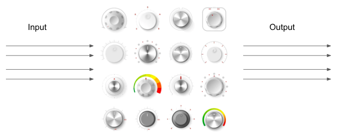
During the training phase of a neural network, we essentially guide it to understand patterns in data. We start by showing the network examples: we say, “Here’s the input, and here’s what we expect the output to be.” Then comes the fascinating part: we adjust/tweak these knobs, so that the network gets better at predicting the correct output for a given input.
As we tweak these knobs, our goal is simple: we want the network to get closer and closer to producing outputs that match our expectations. It’s like fine-tuning an instrument to play the perfect melody. Gradually, through this process, the network starts giving outputs that align more closely with what we anticipate. This adjustment process, known as backpropagation, involves fine-tuning the connections to align the network’s predictions with the provided input-output pairs. For understanding backpropagation better, you can refer to the following blog.
Once our neural network has completed its training phase and learned the knob positions from the examples we provided, it enters the inference phase, where it gets to showcase its newfound skills.
During inference we freeze the adjustments we made to the knobs during training. Think of it as setting the dials to the perfect settings—and now the network is ready to tackle real-world tasks. When we present the network with new data, it springs into action, processing the input and swiftly generating an output based on what it’s learned.
Neural networks are versatile, capable of handling various tasks, from image recognition to natural language processing. By harnessing interconnected neurons, they unlock the potential of artificial intelligence, driving innovation across industries.
For a detailed understanding of how neural networks work, you can refer to the following CloudxLab playlist.
How does model output a word?
Now that we understand the concept of a neural network, let’s delve into its ability to perform classification tasks and how it outputs words.
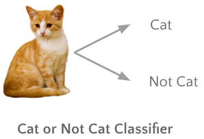
Classification is like sorting things into different groups. Imagine we’re sorting pictures into two categories: pictures of cats and pictures of everything else (not cats). Our job is to teach the computer to look at each picture and decide which category it belongs to. So, when we show it a picture, it’ll say, “Yes, that’s a cat,” or “No, that’s not a cat.” That’s how classification works—it helps computers organize information into clear groups based on what they see.
Outputting a word is also a classification task. Let’s think of a big dictionary with lots of words—say, 50,000 of them. Now, imagine we have a smart computer that’s learning to predict the next word in a sentence. So, when we give it a sequence of words from a sentence, it guesses what word should come next.
But here’s the thing: computers think in numbers, not words. So, we turn each word into a special number, kind of like a token. Then, we train our computer to guess which number (or word) should come next in a sentence. When we give it some words, it looks at all the possibilities in the dictionary and assigns a chance (or probability) to each word, saying which one it thinks is most likely to come next.
Suppose we have the following sequences and their corresponding next words:
- Sequence: “The cat”, Next word: “sat”
- Sequence: “The cat sat”, Next word: “on”
- Sequence: “The cat sat on”, Next word: “the”
- Sequence: “The cat sat on the”, Next word: “mat”
During training, the neural network will learn from these patterns. It will understand that “The cat” is typically followed by “sat”, “The cat sat” is followed by “on”, “The cat sat on” is followed by “the”, and “The cat sat on the” is followed by “mat”. This way, the model learns the language structure and can predict the next word in a sequence based on the learned patterns. After training, our model will be good in predicting the next word in a sentence.
So, our computer’s job is to learn from lots of examples and get really good at guessing the next word in a sentence based on what it’s seen before. It’s like a super smart helper, trying to predict what word you’ll say next in a conversation.
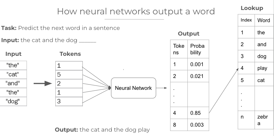
In the above example, we have a dictionary (lookup) of n words. This means the neural network recognizes only these n words from the dictionary and can only produce predictions based on them. Any word not in the dictionary won’t be recognized or generated by the model.
Now, we provide the input “the cat and the dog ___”. We can see that each word is represented by a token in the lookup such as ‘the’ as 1, ‘cat’ as 5, ‘and’ as 2, etc. So we convert our input sequence to tokens using the lookup. Then we pass these tokens to the neural network, and it predicts the probability for each token, representing the chance of that token coming as the next word in the sequence. Then we choose the token with the highest probability, which in our case is token number 4. Upon performing a lookup, we find that token 4 represents the word “play”. So this becomes our output, and the sentence becomes “the cat and the dog play”.
In our example, with a limited vocabulary of ‘n’ words, the neural network can only predict the next word from the provided set of words. However, in large language models like ChatGPT, Bard, etc., the model is trained on a vast corpus of text data containing a diverse range of words and phrases from various sources. By training on a large dataset encompassing a wide vocabulary, the model becomes more proficient at understanding and generating human-like text. It learns the statistical relationships between words, their contexts, and the nuances of language usage across different domains.
When you give LLMs a query or a prompt, they predict the next word in the sequence. Once they generate a word, they then consider what word might come after that, and the process continues until the response is completed. This iterative prediction process allows these models to generate coherent and contextually relevant responses.
Let’s imagine the input prompt provided to ChatGPT is “Write a poem on nature.”Initially, the LLM might predict “The” as the first word. Then, considering “The” as the beginning of the poem, it might predict “beauty” as the next word, leading to “The beauty ____.” Continuing this process, it might predict “of” as the next word, resulting in “The beauty of ____.”
As the LLM predicts each subsequent word, the poem gradually takes shape. It might predict “nature” as the next word, leading to “The beauty of nature ____.” Then, it might predict “is” as the following word, resulting in “The beauty of nature is ____.”
The process continues until the LLM generates a coherent and evocative poem on nature. This iterative approach enables LLMs to create engaging and contextually relevant text based on the given prompt.
Recurrent Neural Networks
Imagine you’re reading a story, and you want to understand what’s happening as you go along. Your brain naturally remembers what you read before and uses that information to understand the story better. That’s kind of how recurrent neural networks work!
In simple terms, RNNs are like brains for computers. They’re really good at processing sequences of data, like words in a sentence or frames in a video. RNNs were introduced in 1980s. What makes them special is that they remember what they’ve seen before and use that memory to make sense of what’s happening next.
So, if you feed a sentence into an RNN, it’ll read one word at a time, just like you read one word after another in a story. But here’s the cool part: as it reads each word, it keeps a memory of what it read before. This memory helps it understand the context of the sentence and make better predictions about what word might come next.
While RNNs were great at processing sequences of data, they struggled with remembering long sequences. So, to address this issue, researchers came up with a special type of RNN called LSTM, which stands for Long Short-Term Memory. LSTMs are like upgraded versions of RNNs—they’re smarter and better at remembering important information from the past.
LSTMs performed better than RNNs to retain memory over long sequences, but still were not very good at the task. To address these challenges, researchers introduced the Transformer model.
For understanding RNNs and LSTMs in detail, you can refer to the following CloudxLab playlist.
Transformer
The introduction of the Transformer marked a significant breakthrough in the field of Natural Language Processing. It emerged in the seminal paper titled “Attention is All You Need.”
The Transformer’s innovative design, leveraging self-attention mechanisms, addressed these shortcomings. By allowing the model to focus on relevant parts of the input sequence, the Transformer could capture long-range dependencies and contextual information more effectively. This breakthrough paved the way for more sophisticated language models, including ChatGPT, that excel in understanding and generating coherent text.
Self-Attention Mechanism
The basic idea: Each time the model predicts an output word, it only uses a part of the input where the most relevant information is concentrated instead of the entire sentence.
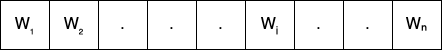
Suppose we have a sentence of n words:-
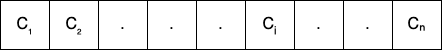
As we know machines only understand number, let’s map these words into vectors:
Now if we take a word vector Cᵢ and we want to compute the similarity of Cᵢ with every other vector, we take dot product of Cᵢ with every other vector in C₁ to Cₙ. If dot product is high, that means vectors are very similar.
To understand about word vectors, embeddings and how dot products represent similarity between two vectors, you can refer to:
These dot products can be big or small, but they’re not really easy to understand on their own. So, we want to make them simpler and easier to compare. To do that, we use a trick called scaling. It’s like putting all these numbers on the same scale, from 0 to 1. This way, we can see which words are more similar to each other. The higher the number, the more similar the words.
Suppose dot(Cᵢ, C₁) is 0.7 and dot(Cᵢ, C₆) is 0.5. Then we can easily say that Cᵢ is more similar to C₁ than to C₆.
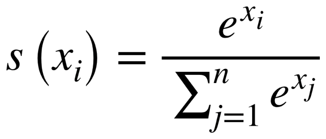
Now, imagine we have these nice numbers, but they’re still not exactly like probabilities (the chances of something happening). So, we use another trick called softmax. It helps us turn these numbers into something that looks more like probabilities.
Softmax basically adjusts the numbers so they all add up to 1, like percentages. This helps the computer understand how important each word is compared to the others. It’s like saying, “Out of all these words, which ones should we pay the most attention to?” Let’s call them attention scores.
Now, we want to use these attention scores to calculate a weighted sum of the original vectors C₁ to Cₙ. This weighted sum is called the context vector, and it gives us a representation of the input sentence that takes into account the importance of each word based on the attention scores. It provides a summary of the sentence that focuses more on the words that are deemed most relevant for the task at hand.
Confused? Let’s understand with an example
Suppose we have input sentence as:- “I love Natural Language Processing“.
Step 1:- Let’s represent each word by encodings. For instance:
“i” = [1, 0, 0, 0, 0]
“love” = [0, 1, 0, 0, 0]
“natural” = [0, 0, 1, 0, 0]
“language” = [0, 0, 0, 1, 0]
“processing” = [0, 0, 0, 0, 1]
Each word in the sentence “I love Natural Language Processing” is first transformed into two types of embeddings:
- Query (Q): This is a representation of the word used to derive attention scores for other words. The Query vector represents the word or token for which we are calculating attention weights concerning other words or tokens in the sequence. For example, if we’re considering the word “love,” the query might be: “What other words help me understand the meaning of ‘love’ in this sentence?”
- Key (K): This is another representation of the word used to compare with other words. It is used to compare with Query vectors during the calculation of attention weights. The key acts like an answer to the query. It tells us how relevant each other word in the sentence is to understanding “love.”
For each word in the input sequence, we first compute the Query (Q) and Key (K) vectors using the initialized weight matrices Wq and Wk as:
Query (Qx) = x * Wq
Key (Kx) = x * Wk

where x is the input encoding, and Wq and Wk are the weight vectors learned during training.
Let’s initialize Wq and Wk with random values. Suppose Wq and Wk is of shape (5, 4). That means the projection dimension of the query and key vector will be 4.
Wq = [[0.94, 0.48, 0.02, 0.93],
     [0.16, 0.72, 0.27, 0.06],
     [0.17, 0.91, 0.6 , 0.21],
     [0.37, 0.85, 0.13, 0.82],
     [0.58, 0.85, 0.13, 0.75]]

Wk = [[0.37, 0.25, 0.17, 0.95],
     [0.56, 0.19, 0.25, 0.91],
     [0.93, 0.01, 0.94, 0.43],
     [0.37, 0.84, 0.59, 0.68],
     [0.97, 0.09, 0.42, 0.73]]
So, for “I”, the query and key vectors come as:
i = [1, 0, 0, 0, 0]
Qi = dot(i, Wq) = [0.94, 0.48, 0.02, 0.93]
Ki = dot(i, Wk) = [0.37, 0.25, 0.17, 0.95]
In the same way, we calculate query and key vectors of all the words, which come as:
Qi = [0.94, 0.48, 0.02, 0.93]
Qlove = [0.16 0.72 0.27 0.06]
Qnatural = [0.17 0.91 0.6 0.21]
Qlanguage = [0.37 0.85 0.13 0.82]
Qprocessing = [0.58 0.85 0.13 0.75]
Ki = [0.37 0.25 0.17 0.95]
Klove = [0.56 0.19 0.25 0.91]
Knatural = [0.93 0.01 0.94 0.43]
Klanguage = [0.37 0.84 0.59 0.68]
Kprocessing = [0.97 0.09 0.42 0.73]
Step 2:– Compute the dot product of query vector of “I”(Qi)with every key vector.
Operation: dot(Qx , Kx), where x is the word. Let’s calculate for “I”. So,
Qi = [0.94, 0.48, 0.02, 0.93]
- dot(Qi , Ki) = 0.94 * 0.37 + 0.48 * 0.25 + 0.02 * 0.17 + 0.93 * 0.95 = 1.35
- dot(Qi , Klove) = 0.94 * 0.56 + 0.48 * 0.19 + 0.02 * 0.25 + 0.93 * 0.91 = 1.47
- dot(Qi , Knatural) = 0.94 * 0.93 + 0.48 * 0.01 + 0.02 * 0.94 + 0.93 * 0.43 = 1.3
- dot(Qi , Klanguage) = 0.94 * 0.37 + 0.48 * 0.84 + 0.02 * 0.59 + 0.93 * 0.68 = 1.4
- dot(Qi , Kprocessing) = 0.94 * 0.97 + 0.48 * 0.09 + 0.02 * 0.42 + 0.93 * 0.73 = 1.64
Dot product vector w.r.t I = [1.35, 1.47, 1.3, 1.4, 1.64]
In the same way, we calculate dot product vector of all the query vectors with key vectors.
Dot product vector w.r.t I (scorei) = [1.35, 1.47, 1.3, 1.4, 1.64]
Dot product vector w.r.t love (scorelove) = [0.34, 0.35, 0.44, 0.86, 0.38]
Dot product vector w.r.t natural (scorenatural) = [0.59, 0.61, 0.82, 1.32, 0.65]
Dot product vector w.r.t language (scorelanguage) = [1.15, 1.15, 0.83, 1.49, 1.09]
Dot product vector w.r.t processing (scoreprocessing) = [1.16, 1.2, 0.99, 1.52, 1.24]
But these scores can vary widely in magnitude and lack a clear interpretation of relative importance among the elements in the sequence.
Here comes Softmax to rescue.
Softmax function is applied to the attention scores to convert them into probabilities.
This transformation has two main effects:
- Amplifying Higher Scores:
- Scores that are initially higher are amplified more by the exponential function in the softmax numerator.
- Diminishing Lower Scores:
- Scores that are lower initially receive smaller weights after softmax normalization.
Let’s understand it with an example.
# Let’s take an array:
arr = [1,2,3,4,5,6]
Let’s calculate the softmax distribution:
import numpy as np
numerator = np.exp(arr) = [ 2.71828183, 7.3890561 , 20.08553692, 54.59815003, 148.4131591 , 403.42879349]

denominator = sum(numerator) = 636.6329774790333

softmax = numerator/denominator = [0.00426978, 0.01160646, 0.03154963, 0.08576079, 0.23312201,
0.63369132]
Now, let’s we plot the bar graph of original array and softmax array.
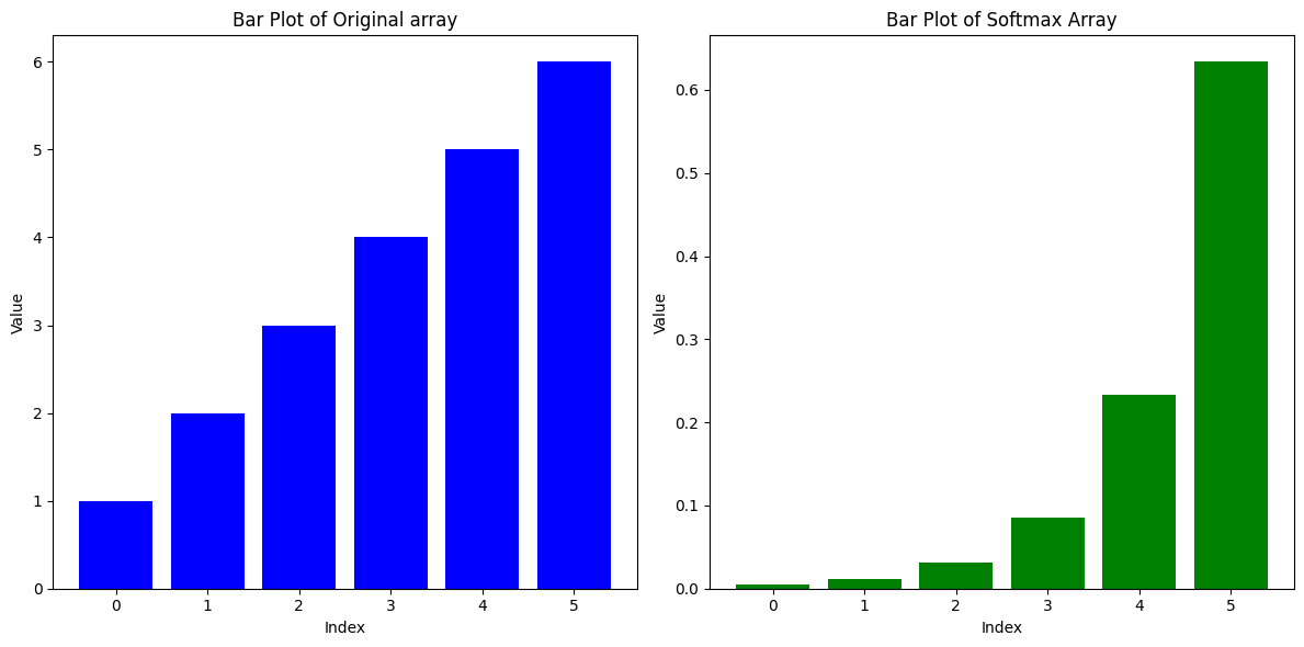
In the above image we can see that it amplified the higher scores, and diminished the lower scores.
Now, we will pass the calculated attention scores to the softmax function.
But, dot products grow large in magnitude, where the application of the softmax function would then return extremely small gradients.
What can be done to bring scores to a definite scale?
Yes, you are right. Scaling. Before passing the scores to softmax, we will first scale them.
Step 3:– Scale the attention scores.
We simply divide the vectors with square root of length of the k vector, which we calculated. The length of our k vector is 4, so we’ll divide the dot product vectors with sqrt(4), which is 2.
scorei = [1.35, 1.47, 1.3, 1.4, 1.64] / 2 = [0.68, 0.74, 0.65, 0.7 , 0.82]
scorelove = [0.34, 0.35, 0.44, 0.86, 0.38] / 2= [0.17, 0.18, 0.22, 0.43, 0.19]
scorenatural = [0.59, 0.61, 0.82, 1.32, 0.65] / 2 = [0.3 , 0.3 , 0.41, 0.66, 0.32]
scorelanguage = [1.15, 1.15, 0.83, 1.49, 1.09] / 2 = [0.57, 0.57, 0.42, 0.74, 0.55]
scoreprocessing = [1.16, 1.2, 0.99, 1.52, 1.24] / 2 = [0.58, 0.6 , 0.5 , 0.76, 0.62]
Step 4:– Apply softmax
After applying softmax, our scores come as:
scorei = [0.19, 0.2 , 0.19, 0.2 , 0.22]
scorelove = [0.19, 0.19, 0.2 , 0.24, 0.19]
scorenatural = [0.18, 0.18, 0.2 , 0.26, 0.18]
scorelanguage = [0.2 , 0.2 , 0.17, 0.24, 0.2 ]
scoreprocessing = [0.19, 0.2 , 0.18, 0.23, 0.2 ]
Step 5: Project context vector
Now we are just one step away from getting our final attention scores. We have to decide that in how many dimensions should we represent each word. For that we use Value embedding.
We calculate the Value embeddings in the same way we calculated Query(Q) and Key(K) embeddings, i.e. V = x * Wv.
So, for value embeddings, let’s take Wv of shape (5,8). That means, we want to represent the context vector of each word with 8 dimensions.
Wv = [[0.71, 0.95, 0.32, 0.16, 0.79, 0.61, 0.63, 0.06],
      [0.6 , 0.84, 0.26, 0.29, 0.88, 0.26, 0.11, 0.6 ],
      [0.65, 0.78, 0.02, 0.18, 0.07, 0.67, 0.58, 0.46],
      [0.39, 0.68, 0.09, 0.23, 0.89, 0.14, 0.83, 0.64],
      [0.7 , 0.96, 0.22, 0.45, 0.65, 0.79, 0.01, 0.59]]
So, our Value(V) matrix comes as: V = x * Wv
V = [[0.71, 0.95, 0.32, 0.16, 0.79, 0.61, 0.63, 0.06],
     [0.6 , 0.84, 0.26, 0.29, 0.88, 0.26, 0.11, 0.6 ],
     [0.65, 0.78, 0.02, 0.18, 0.07, 0.67, 0.58, 0.46],
     [0.39, 0.68, 0.09, 0.23, 0.89, 0.14, 0.83, 0.64],
     [0.7 , 0.96, 0.22, 0.45, 0.65, 0.79, 0.01, 0.59]]
Now, we simply multiply the attention scores with Value matrix to get out final context vector.
Context vector of I comes as:
Operation: np.matmul(scorex , V), where x is the word.
import numpy as np

Context["I"] = np.matmul(scorei , V) = [0.61, 0.85, 0.18, 0.27, 0.66, 0.5 , 0.42, 0.48]
Context vector of I = [0.61, 0.85, 0.18, 0.27, 0.66, 0.5 , 0.42, 0.48]
In the same way, we calculate context vector of all the words.
Context vector of I = [0.61, 0.85, 0.18, 0.27, 0.66, 0.5 , 0.42, 0.48]
Context vector of love = [0.6 , 0.83, 0.18, 0.26, 0.66, 0.48, 0.45, 0.48]
Context vector of natural = [0.59, 0.83, 0.17, 0.26, 0.66, 0.47, 0.46, 0.48]
Context vector of language = [0.6 , 0.84, 0.18, 0.26, 0.68, 0.47, 0.44, 0.48]
Context vector of processing = [0.6 , 0.84, 0.18, 0.26, 0.67, 0.48, 0.44, 0.48]
This context vector combines the original embedding of the word with information about how it relates to other words in the sentence, all based on the calculated attention scores.
Now the question arises, why have we done all this?
As words, vectors don’t tell the relationship of a particular word with other words of the sentence, so it is not any better than a random subset of words. As we know, sentence is a group of words which makes sense. So we calculate their context vector which also keep the information about the relationship of the word with every other word. This is called self-attention mechanism.
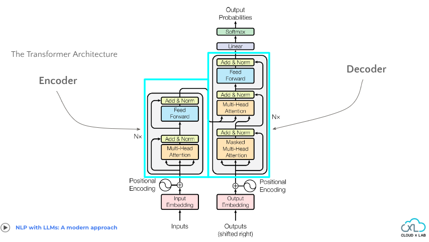
Transformer architecture
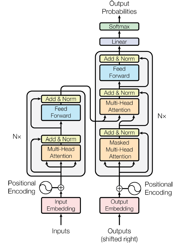
The transformer architecture is made of two blocks: Encoder(left) and Decoder(right). These encoder and decoder blocks are stacked N times.
Encoder:
- Functionality: The encoder’s goal is to extract meaningful features and patterns from the input sequence, which can then be used by the decoder for generating the output sequence. It analyzes the input sequence, token by token, and generates contextualized representations for each token. These representations capture information about the token’s context within the input sequence.
- Input: The encoder receives the input sequence, typically represented as a sequence of word embeddings or tokens.
- Output: The encoder outputs a sequence of contextualized representations for each token in the input sequence.
Decoder:
- Functionality: The decoder block is tasked with generating the output sequence based on the contextualized representations provided by the encoder. It’s task is to predict the next token in the output sequence based on the context provided by the encoder and the previously generated tokens. It generates the output sequence token by token, taking into account the learned representations and the context provided by the encoder.
- Input: Initially, the decoder receives the same sequence of contextualized representations generated by the encoder.
- Outputs(Shifted right): During training, the decoder also receives a shifted version of the output sequence, where each token is shifted to the right by one position. This shifted sequence is used for teacher forcing, helping the decoder learn to predict the next token in the sequence based on the previous tokens.
- Output: The decoder generates the output sequence, which represents the model’s predictions or translations.
Positional Encoding
Consider the 2 following sentences:
> I do not like the story of the movie, but I do like the cast
> I do like the story of the movie, but I do not like the cast
What is the difference between these 2 sentences?
The words are same but the meaning is different. This shows that information of order is required to distinguish different meanings
Positional embedding generates embeddings which allows the model to learn the relative positions of words.
Now, as we have a brief overview of how the transformer works, let’s cover the components inside encoder and decoder blocks one by one. We’ll simultaneously code the components which will give us the final code of GPT.
Coding GPT from scratch
Let’s code it. Make sure you are comfortable with Tensorflow and Keras as we will be using it. You can access the complete code used in this blog at https://github.com/cloudxlab/GPT-from-scratch/tree/master. We will be coding only the decoder part of the transformer, as modern LLMs such as ChatGPT only use the decoder part of the transformer.
Head(attention) block
So, we’ll start with implementing the Head block. In the context of transformer-based architectures, a “Head” refers to a distinct computational unit responsible for performing attention computations. It operates within the broader framework of self-attention, allowing the model to focus on relevant parts of the input sequence.
Let’s start with writing the __init__() method that sets up the necessary components and parameters required for attention computations.
class Head(tf.keras.layers.Layer):
    """ one head of self-attention """

    def __init__(self, head_size):
        super(Head, self).__init__()
        self.key = tf.keras.layers.Dense(head_size, use_bias=False)
        self.query = tf.keras.layers.Dense(head_size, use_bias=False)
        self.value = tf.keras.layers.Dense(head_size, use_bias=False)

        tril = tf.linalg.band_part(tf.ones((block_size, block_size)), -1, 0)
        self.tril = tf.constant(tril)

        self.dropout = tf.keras.layers.Dropout(dropout)
In the above code,
- The
key,query, andvaluelayers are initialized as dense layers using thetf.keras.layers.Densemodule. By initializing these layers without biases (use_bias=False), the model learns to capture complex relationships and patterns within the input sequence. - A lower triangular mask (
tril) is generated usingtf.linalg.band_part. This mask is essential for preventing the model from attending to future tokens during training, thereby avoiding information leakage. The lower triangular mask ensures that each position in the input sequence can only attend to positions/words preceding it. While training transformers, we pass the whole input sequence at once. So suppose, we have the following input sequence:
[<start>, I, love, natural, language, processing, <end>]
Now here we want to predict the word after “natural”. The lower triangular mask ensures that during training, our model can only attend to tokens that precede “natural” (i.e., <start>, ‘I’, ‘love’), masking out the words that come after it. This prevents the model from accessing future tokens, preserving the autoregressive nature of the task and ensuring that predictions are based solely on preceding context. It is only used in the decoder block and not the encoder block as while encoding we can access all the words but while decoding we cannot, because our task is to predict the next word.
- In the end, we use a dropout layer initialized using
tf.keras.layers.Dropout. Dropout regularization is applied to the attention weights during training to prevent overfitting and improve generalization performance.
Now, we will code the attention mechanism.
def call(self, x):
        # input of size (batch, time-step, channels)
        # output of size (batch, time-step, head size)
        B, T, C = x.shape
        k = self.key(x)   # (B, T, hs)
        q = self.query(x) # (B, T, hs)

        # compute attention scores ("affinities")
        wei = tf.matmul(q, tf.transpose(k, perm=[0, 2, 1])) * tf.math.rsqrt(tf.cast(k.shape[-1], tf.float32))  # (B, T, T)
        wei = tf.where(self.tril[:T, :T] == 0, float('-inf'), wei)  # (B, T, T)
        wei = tf.nn.softmax(wei, axis=-1)  # (B, T, T)
        wei = self.dropout(wei)

        # perform the weighted aggregation of the values
        v = self.value(x)  # (B, T, hs)
        out = tf.matmul(wei, v)  # (B, T, T) @ (B, T, hs) -> (B, T, hs)
        return out
- The method receives input
x, which is a tensor representing the input sequence. It assumes that the input has three dimensions:(batch_size, time_steps, channels).
- Batch Size: It’s the number of sequences processed together. For instance, if we process 32 movie reviews simultaneously, the batch size is 32.
- Time Steps: It’s the length of each sequence. In a movie review consisting of 100 words, each word is a time step.
- Channels: It’s the dimensionality of each feature in a sequence. If we represent words with 300-dimensional embeddings, each word has 300 channels.
- Then it applies the
keyandquerylayers to the input tensorx, resulting in tensorskandq, both with shapes(batch_size, time_steps, head_size). Herehead_sizerefers to the dimensionality of the feature space within each attention head. For example, ifhead_sizeis set to 64, it means that each attention head operates within a feature space of dimension 64. - It computes attention scores between the query and key tensors
(q, k)using the dot product followed by normalization. The result is a tensorweiof shape(batch_size, time_steps, time_steps), where each element represents the attention score between a query and a key. - The lower triangular mask is applied to
weito prevent attending to future tokens, ensuring the autoregressive property of the model. - The softmax function is then applied along the last dimension to obtain attention weights, ensuring that the weights sum up to 1 for each time step.
- After that, Dropout regularization is applied to the attention weights to prevent overfitting during training.
- Then it applies the
valuelayer to the input tensorx, resulting in a tensorvof shape(batch_size, time_steps, head_size). It performs a weighted sum of the value tensorvusing the attention weightswei, resulting in the output tensoroutof shape(batch_size, time_steps, head_size). This step computes the context vector, which represents the contextually enriched representation of the input sequence based on attention computations.
The Head block we implemented represents a single attention head within the Transformer architecture. It performs attention computations, including key, query, and value projections, attention score calculation, masking, softmax normalization, and weighted aggregation of values. Each Head block focuses on capturing specific patterns and relationships within the input sequence, contributing to the overall representation learning process of the model.
Now, let’s delve into the concept of multi-head attention.
Multi-Head attention Block
Multi-head attention is a key component of the Transformer architecture designed to enhance the model’s ability to capture diverse patterns and dependencies within the input sequence. Instead of relying on a single attention head, the model utilizes multiple attention heads in parallel. Each attention head learns different patterns and relationships within the input sequence independently. The outputs of the multiple attention heads are then concatenated or combined in some way to produce a comprehensive representation of the input sequence.
Why multi-head attention?
- Capturing Diverse Patterns: Each attention head specializes in capturing specific patterns or dependencies within the input sequence, enhancing the model’s capacity to learn diverse relationships.
- Improved Representation Learning: By leveraging multiple attention heads, the model can capture complex and nuanced interactions within the data, leading to more expressive representations.
- Enhanced Robustness: Multi-head attention enables the model to learn from different perspectives simultaneously, making it more robust to variations and uncertainties in the input data.
Now, let’s code the multi-head attention.
class MultiHeadAttention(tf.keras.layers.Layer):
    """ multiple heads of self-attention in parallel """

    def __init__(self, num_heads, head_size):
        super(MultiHeadAttention, self).__init__()
        self.heads = [Head(head_size) for _ in range(num_heads)]
        self.proj = tf.keras.layers.Dense(n_embd)
        self.dropout = tf.keras.layers.Dropout(dropout)

    def call(self, x):
        out = tf.concat([h(x) for h in self.heads], axis=-1)
        out = self.dropout(self.proj(out))
        return out
Initialization:
num_headsandhead_sizeare parameters passed to initialize theMultiHeadAttentionlayer.num_headsspecifies the number of attention heads to be used in parallel andhead_sizedetermines the dimensionality of the feature space within each attention head.
__init__ Method:
- In the
__init__method, we initialize the multiple attention heads by creating a list comprehension ofHeadinstances. EachHeadinstance represents a single attention head with the specifiedhead_size. - Additionally, we initialize a projection layer (
self.proj) to aggregate the outputs of the multiple attention heads into a single representation. - A dropout layer (
self.dropout) is also initialized to prevent overfitting during training.
call Method:
- The
callmethod takes the input tensorxand processes it through each attention head in parallel. - For each attention head in
self.heads, the input tensorxis passed through the attention head, and the outputs are concatenated along the last axis usingtf.concat. - The concatenated output is then passed through the projection layer
self.projto combine the information from multiple heads into a single representation. - Finally, dropout regularization is applied to the projected output to prevent overfitting.
In summary, the MultiHeadAttention class encapsulates the functionality of performing self-attention across multiple heads in parallel, enabling the model to capture diverse patterns and relationships within the input sequence. It forms a critical building block of the Transformer architecture, contributing to its effectiveness in various natural language processing tasks.
Feed-forward layer
The FeedForward layer in the Transformer architecture introduces non-linearity and feature transformation, essential for capturing complex patterns in the data. Through the ReLU activation function, it models non-linearities, aiding better representation learning. By projecting input features into higher-dimensional spaces and reducing dimensionality, it enhances the model’s ability to capture intricate dependencies and structures, fostering more expressive representations. Additionally, dropout regularization within the layer prevents overfitting by encouraging robust and generalizable representations, improving the model’s performance across diverse natural language processing tasks.
class FeedForward(tf.keras.layers.Layer):
    """ a simple linear layer followed by a non-linearity """

    def __init__(self, n_embd):
        super(FeedForward, self).__init__()
        self.net = tf.keras.Sequential([
            tf.keras.layers.Dense(4 * n_embd),
            tf.keras.layers.ReLU(),
            tf.keras.layers.Dense(n_embd),
            tf.keras.layers.Dropout(dropout),
        ])

    def call(self, x):
        return self.net(x)
- The
FeedForwardlayer is initialized with the parametern_embd, which specifies the dimensionality of the input and output feature spaces, or we can say shape of input and output tensor.
__init__ Method:
- In the
__init__method, we define a simple feedforward neural network usingtf.keras.Sequential. - The network consists of two dense layers:
- The first dense layer (
tf.keras.layers.Dense(4 * n_embd)) projects the input features into a higher-dimensional space, followed by a rectified linear unit (ReLU) activation function (tf.keras.layers.ReLU()). - The second dense layer (
tf.keras.layers.Dense(n_embd)) reduces the dimensionality back to the original feature space.
- The first dense layer (
- Additionally, dropout regularization is applied using
tf.keras.layers.Dropout(dropout)to prevent overfitting during training.
call Method:
- The
callmethod takes the input tensorxand passes it through the feedforward neural network defined inself.net. The output of the feedforward network is returned as the final result.
In summary, the FeedForward class implements a feedforward neural network layer within the Transformer architecture. It applies linear transformations followed by non-linear activations to process input features, enabling the model to capture complex patterns and relationships within the data. This layer contributes to the expressive power and effectiveness of the Transformer model in various natural language processing tasks.
Transformer Block
Now, let’s add all these components to form a transformer block
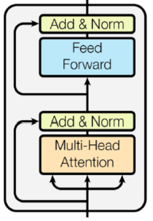
class Block(tf.keras.layers.Layer):
    """ Transformer block: communication followed by computation """

    def __init__(self, n_embd, n_head):
        super(Block, self).__init__()
        head_size = n_embd // n_head
        self.sa = MultiHeadAttention(n_head, head_size)
        self.ffwd = FeedForward(n_embd)
        self.ln1 = tf.keras.layers.LayerNormalization(epsilon=1e-6)
        self.ln2 = tf.keras.layers.LayerNormalization(epsilon=1e-6)

    def call(self, x):
        x = x + self.sa(self.ln1(x))
        x = x + self.ffwd(self.ln2(x))
        return x
- The
Blockclass is initialized with two parameters:n_embdandn_head.n_embdspecifies the dimensionality of the input and output feature spaces andn_headdetermines the number of attention heads to be used in the MultiHeadAttention layer. - Inside the
__init__method, we initialize the components of the Transformer block: MultiHeadAttention (self.sa), FeedForward (self.ffwd): Layer Normalization (self.ln1,self.ln2), represented by Add&Norm in the above diagram. - The
callmethod of theBlockclass in the Transformer architecture processes the input tensorxthrough a series of transformations. Firstly, the input tensor undergoes the MultiHeadAttention layer (self.sa), followed by Layer Normalization (self.ln1). The resulting output is then added to the original input tensor to facilitate communication between different positions in the sequence. Subsequently, the augmented tensor from the previous step is passed through the FeedForward layer(self.ffwd), followed by another Layer Normalization (self.ln2). The output of the feedforward computation is again added to the augmented tensor.
GPT
Now, as we have designed the components of GPT, let’s stack them together to build our GPT.
class GPTLanguageModel(tf.keras.Model):

    def __init__(self):
        super(GPTLanguageModel, self).__init__()
        # each token directly reads off the logits for the next token from a lookup table
        self.token_embedding_table = tf.keras.layers.Embedding(vocab_size, n_embd)
        self.position_embedding_table = tf.keras.layers.Embedding(block_size, n_embd)
        self.blocks = tf.keras.Sequential([Block(n_embd, n_head=n_head) for _ in range(n_layer)])
        self.ln_f = tf.keras.layers.LayerNormalization(epsilon=1e-6)
        self.lm_head = tf.keras.layers.Dense(vocab_size, kernel_initializer='normal', bias_initializer='zeros')
The GPTLanguageModel class defines a language model based on the Generative Pre-trained Transformer (GPT) architecture.
__init__ Method:
- The __init__ method initializes the components necessary for the GPT language model.
self.token_embedding_table: This layer converts input tokens into dense vectors of fixed size (embedding vectors). Each token is mapped to a unique embedding vector in a lookup table.self.position_embedding_table: This layer generates position encodings that represent the position of each token in the input sequence.self.blocks: A sequence of Transformer blocks responsible for processing the input sequence. Each block comprises multi-head self-attention mechanisms and feedforward neural networks.self.ln_f: Applies layer normalization to the final hidden states of the Transformer blocks. It stabilizes the training process by ensuring consistent distributions of hidden states across layers.self.lm_head: A dense layer that maps the final hidden states of the Transformer blocks to logits over the vocabulary. Logits represent unnormalized probabilities of each token in the vocabulary being the next token in the sequence.
Let’s see these components in the transformer architecture.
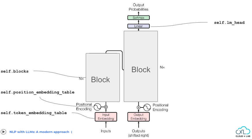
Note:- The self.ln_f is not explicitly shown in the image.
Now let’s write the method which will perform the forward pass during our training phase.
call Method:
def call(self, idx, targets=None):
        B, T = idx.shape

        # idx and targets are both (B,T) tensor of integers
        tok_emb = self.token_embedding_table(idx)  # (B,T,C)
        pos_emb = self.position_embedding_table(tf.range(T, dtype=tf.float32))  # (T,C)
        x = tok_emb + pos_emb  # (B,T,C)
        x = self.blocks(x)  # (B,T,C)
        x = self.ln_f(x)  # (B,T,C)
        logits = self.lm_head(x)  # (B,T,vocab_size)

        if targets is None:
            loss = None
        else:
            B, T, C = logits.shape
            logits = tf.reshape(logits, (B * T, C))
            targets = tf.reshape(targets, (B * T,))
            loss = tf.keras.losses.SparseCategoricalCrossentropy(from_logits=True)(targets, logits)

        return logits, loss
- The call method takes idx and targets as input.
idxrepresents the input tensor containing integer indices of tokens. It has shape (batch_size, sequence_length).targetsrepresents the target tensor containing the indices of the tokens to be predicted. It has the same shape asidx.
tok_embretrieves the token embeddings for the input indices from the token embedding table.pos_embgenerates position embeddings for each position in the input sequence using the position embedding table.- x = tok_emb + pos_emb: The token and position embeddings are added together to incorporate both token and positional information into the input representation
x. - x = self.blocks(x): Then the input representation
xis passed through the Transformer blocks (self.blocks), which process the sequence and extract relevant features. - x = self.ln_f(x): Layer normalization (
self.ln_f) is applied to stabilize the training process by normalizing the hidden states of the Transformer blocks. - logits = self.lm_head(x): The final hidden states are passed through the output layer (
self.lm_head), which generates logits for each token in the vocabulary. - If
targetsare provided, the method computes the loss using the sparse categorical cross-entropy loss function. It reshapes the logits and targets tensors to match the format required by the loss function. - If
targetsare not provided, the loss is set to None. That means we are not training the model but using it for prediction/text generation. - The method returns the logits and the computed loss (if applicable).
Now that we’ve explored the inner workings of the call method, let’s dive into another captivating feature of our Generative Pre-trained Transformer (GPT): the generate method. While the call method focuses on predicting the next character given a sequence, the generate method takes it a step further by generating entire sequences of text. It relies on the call method internally to predict each subsequent character, iteratively building the complete sequence.
generate Method:
def generate(self, idx, max_new_tokens):
        # idx is (B, T) array of indices in the current context
        for _ in range(max_new_tokens):
            # crop idx to the last block_size tokens
            idx_cond = idx[:, -block_size:]
            # get the predictions
            logits, loss = self(idx_cond)
            # focus only on the last time step
            logits = logits[:, -1, :]  # becomes (B, C)
            # apply softmax to get probabilities
            probs = tf.nn.softmax(logits, axis=-1)  # (B, C)
            # sample from the distribution
            idx_next = tf.random.categorical(tf.math.log(probs), num_samples=1, dtype=tf.int64)  # (B, 1)
            # append sampled index to the running sequence
            idx = tf.concat([idx, idx_next], axis=1)  # (B, T+1)
        return idx
- for _ in range(max_new_tokens): The method iterates for a specified number of
max_new_tokensto generate new tokens based on the provided input sequenceidx. max_new_tokens tells us about the number of tokens we want our GPT to generate. - idx_cond = idx[:, -block_size:]: Then it extracts the last
block_sizetokens from the input sequenceidxto ensure that the model generates new tokens based on the most recent context. This cropping operation ensures that the model’s predictions are influenced by the most recent tokens. - logits, loss = self(idx_cond): Then the method invokes the model’s
callmethod with the cropped input sequenceidx_condto obtain predictions for the next token in the sequence. The model generates logits, which are unnormalized probabilities, for each token in the vocabulary. - logits = logits[:, -1, :]: It selects only the logits corresponding to the last time step of the sequence, representing predictions for the next token to be generated. This step ensures that the model focuses on predicting the next token based on the most recent context.
- probs = tf.nn.softmax(logits, axis=-1): Softmax activation is applied to the logits to convert them into probabilities. This softmax operation ensures that the model’s predictions are transformed into a probability distribution over the vocabulary, indicating the likelihood of each token being the next token in the sequence.
- idx_next = tf.random.categorical(tf.math.log(probs), num_samples=1, dtype=tf.int64): It samples tokens from the probability distribution using the
tf.random.categoricalfunction, which randomly selects one token index from the probability distribution for each sequence in the batch. Thelog(probs)argument is used to stabilize the sampling process. - idx = tf.concat([idx, idx_next], axis=1): Then the sampled token indices are appended to the original input sequence
idx, extending the sequence with the newly generated tokens. - This process repeats for each iteration of the loop, generating new tokens until the desired number of tokens (
max_new_tokens) is reached. - Finally, the method returns the updated input sequence
idx, which now includes the newly generated tokens, representing an extended sequence with additional context and predictions for future tokens.for _ in range(max_new_tokens):
In summary, the Generative Pre-trained Transformer (GPT) architecture employs advanced techniques like multi-head self-attention, feedforward neural networks, and layer normalization to understand and generate natural language text. With token and position embedding tables and a stack of Transformer blocks, GPT captures complex language patterns effectively.
Now, it’s time to train the GPT model on relevant datasets, fine-tune its parameters, and explore its capabilities across different tasks and domains. We’ll use the Shakespear dataset to train our GPT. This means our model will learn to generate text in the style of Shakespeare’s writings. You can find the dataset at https://github.com/cloudxlab/GPT-from-scratch/blob/master/input.txt.
Let’s start with loading the dataset:
Loading the data
with open('input.txt', 'r', encoding='utf-8') as f:
    text = f.read()
Now, let’s create the character mappings so that we can convert the characters into numbers to feed it to machine.
chars = sorted(list(set(text)))
vocab_size = len(chars)
stoi = {ch: i for i, ch in enumerate(chars)}
itos = {i: ch for i, ch in enumerate(chars)}
encode = lambda s: [stoi[c] for c in s]
decode = lambda l: ''.join([itos[i] for i in l])
The above code initializes dictionaries for character-to-index and index-to-character mappings:
- It extracts unique characters from the text and sorts them alphabetically.
- Two dictionaries are created:
stoi: Maps characters to indices.itos: Maps indices to characters.
- Encoding (
encode) and decoding (decode) functions are defined to convert between strings and lists of indices.
Now let’s divide our dataset into training and testing set.
# Train and test splits
data = tf.constant(encode(text), dtype=tf.int64)
n = int(0.9 * len(data))
train_data = data[:n]
val_data = data[n:]
To streamline our data processing, we’ll break it down into manageable batches. This approach helps us efficiently handle large datasets without overwhelming our system resources. Let’s write a function to load our data in batches, enabling us to feed it into our model systematically and effectively.
# Data loading into batches
def get_batch(split):
    data_split = train_data if split == 'train' else val_data
    ix = tf.random.uniform(shape=(batch_size,), maxval=len(data_split) - block_size, dtype=tf.int32)
    x = tf.stack([data_split[i:i+block_size] for i in ix])
    y = tf.stack([data_split[i+1:i+block_size+1] for i in ix])
    return x, y
Now that we have our dataset ready, we need a function to calculate the loss. This loss function helps us understand how well our model is performing during training. By evaluating the loss, we can adjust our model’s weights using the backpropagation algorithm, which fine-tunes its parameters to minimize the loss and improve performance over time. Let’s craft a simple yet effective function to calculate the loss for our model.
Calculating Loss
# Calculating loss of the model
def estimate_loss(model):
    out = {}
    model.trainable = False
    for split in ['train', 'val']:
        losses = tf.TensorArray(tf.float32, size=eval_iters)
        for k in range(eval_iters):
            X, Y = get_batch(split)
            logits, loss = model(X, Y)
            losses = losses.write(k, loss)
        out[split] = losses.stack().numpy().mean()
    model.trainable = True
    return out
- The function starts by initializing an empty dictionary named
outto store the loss values for both the training and validation splits. - It sets the
trainableattribute of the model toFalseto ensure that the model’s parameters are not updated during the loss estimation process. - The function iterates over two splits: ‘train’ and ‘val’, representing the training and validation datasets, respectively.
- Within each split, the function iterates
eval_iterstimes. In each iteration, it retrieves a batch of input-output pairs (X, Y) using theget_batch(split)function. - For each batch, the model is called with inputs X and targets Y to obtain the logits and the corresponding loss.
- The loss value for each iteration is stored in a TensorFlow TensorArray named
losses. - Once all iterations for a split are completed, the mean loss value across all iterations is computed using the
numpy().mean()method, and it is stored in theoutdictionary with the corresponding split key. - After iterating over both ‘train’ and ‘val’ splits, the model’s
trainableattribute is set back toTrueto allow further training if needed. - Finally, the function returns the dictionary
out, containing the average loss values for both the training and validation splits.
Training the model
Now, let’s define the hyperparameters needed to configure our model training.
# hyperparameters
batch_size = 64
block_size = 256
max_iters = 5000
eval_interval = 500
learning_rate = 3e-4
eval_iters = 200
n_embd = 384
n_head = 6
n_layer = 6
dropout = 0.2

# Set random seed
tf.random.set_seed(1337)
Now, let’s implement the training loop for our model. This loop iterates through the dataset, feeding batches of data to the model for training. Within each iteration, the model calculates the loss and updates its weights using the backpropagation algorithm. By repeating this process over multiple epochs, our model gradually learns to make accurate predictions and improve its performance. Let’s dive in and code the training loop for our model.
#Training the model. GPU is recommended for training.

model = GPTLanguageModel()
optimizer = tf.keras.optimizers.Adam(learning_rate)

for iter in range(max_iters):

    # every once in a while evaluate the loss on train and val sets
    if iter % eval_interval == 0 or iter == max_iters - 1:
        losses = estimate_loss(model)
        print(f"step {iter}: train loss {losses['train']:.4f}, val loss {losses['val']:.4f}")

    # sample a batch of data
    xb, yb = get_batch('train')

    # evaluate the loss
    with tf.GradientTape() as tape:
        logits, loss = model(xb, yb)

    grads = tape.gradient(loss, model.trainable_variables)
    optimizer.apply_gradients(zip(grads, model.trainable_variables))
- The
GPTLanguageModelclass is instantiated, creating an instance of the GPT language model. - Then an Adam optimizer is initialized with the specified learning rate (
learning_rate). - The training loop iterates over a specified number of iterations (
max_iters). During each iteration, the model’s performance is periodically evaluated on both the training and validation datasets. - In each iteration, a batch of data (
xb,yb) is sampled from the training dataset using theget_batchfunction. This function retrieves input-output pairs for training. - The loss is computed by forward-passing the input batch (
xb) through the model (model) and comparing the predictions with the actual targets (yb). - A gradient tape (
tf.GradientTape) records operations for automatic differentiation, enabling the computation of gradients with respect to trainable variables. - Gradients of the loss with respect to the trainable variables are computed using
tape.gradient. - The optimizer (
optimizer) then applies these gradients to update the model’s trainable parameters using the Adam optimization algorithm.
With the completion of the training loop, our model has been trained using gradient descent optimization. Through iterations of parameter updates, it has learned to minimize the loss function, improving its ability to generate coherent and contextually relevant text. This training process equips the model with the knowledge and understanding necessary to perform various natural language processing tasks effectively.
step 0: train loss 4.5158, val loss 4.5177
step 500: train loss 1.9006, val loss 2.0083
step 1000: train loss 1.4417, val loss 1.6584
step 1500: train loss 1.2854, val loss 1.5992
step 2000: train loss 1.1676, val loss 1.5936
step 2500: train loss 1.0419, val loss 1.6674
step 3000: train loss 0.9076, val loss 1.8094
step 3500: train loss 0.7525, val loss 2.0218
step 4000: train loss 0.6012, val loss 2.3162
step 4500: train loss 0.4598, val loss 2.6565
step 4999: train loss 0.3497, val loss 2.9876
From the provided training log, we can observe several key insights:
- Training Progress: As the training progresses, both the training loss and validation loss decrease gradually. This indicates that our model is learning and improving its performance over time.
- Overfitting: Towards the end of the training process, we notice a discrepancy between the training loss and the validation loss. While the training loss continues to decrease, the validation loss starts to increase after a certain point. This divergence suggests that our model may be overfitting to the training data, performing well on the training set but struggling to generalize to unseen data represented by the validation set.
- Model Performance: The final validation loss provides insight into the overall performance of our model. A lower validation loss indicates better generalization and performance on unseen data. In this case, the validation loss seems relatively high, suggesting that our model may not be performing optimally.
Now, it’s important to note that the observed behavior in the training log, including the increasing validation loss towards the end of training, was intentionally introduced to highlight the phenomenon of overfitting. Overfitting occurs when a model learns to perform well on the training data but struggles to generalize to unseen data.
As part of your learning journey, it’s now your homework to address this issue and improve the model’s performance. You can explore various strategies to combat overfitting, such as adjusting the model architecture, incorporating regularization techniques, or increasing the diversity of the training data.
We have saved the weights of the model after 5000 iteration. You can directly use those to avoid the training phase as it can take a lot of time without GPU. The weights are present at: https://github.com/cloudxlab/GPT-from-scratch/blob/master/gpt_model_weights.h5.
# Initializing model with pre-trained weights. Use this if you don't want to re-train the model.
model = GPTLanguageModel()
dummy_input = tf.constant([[0]], dtype=tf.int32)
model(dummy_input)
model.load_weights('gpt_model_weights.h5')
Now we will generate new text using the model.
# generate from the model
context = tf.zeros((1, 1), dtype=tf.int64)
generated_sequence = model.generate(context, max_new_tokens=500).numpy()
print(decode(generated_sequence[0]))
- An initial context is set up using
tf.zeros((1, 1), dtype=tf.int64). This initializes a tensor of shape(1, 1)with all elements set to zero, indicating the starting point for text generation. - The
generatemethod of the trained model (model) is called to generate new text sequences based on the provided initial context. Themax_new_tokensparameter specifies the maximum number of new tokens to generate in the text sequence. - The generated sequence is then decoded using a decoding function (
decode) to convert the sequence of token IDs into human-readable text.
So, the output is:
Now keeps.
Can I know should thee were trans--I protest,
To betwixt the Samart's the mutine.

CAMILLO:
Ha, madam!
Sir, you!
You pitiff now, but you are worth aboards,
Betwixt the right of your ox adversaries,
Or let our suddenly in all severaltius free
Than Bolingbroke to England. Mercutio,
Ever justice with his praisence, he was proud;
When she departed by his fortune like a greer,
And in the gentle king fair hateful man.
Farewell; so old Cominius, away; I rather,
To you are therefore be behold
The generated text exhibits a level of coherence and structure reminiscent of Shakespearean language, suggesting that the model has effectively learned patterns from the Shakespearean text data it was trained on. The text includes elements such as archaic language, poetic imagery, and character interactions, which are characteristic of Shakespeare’s writing style.
Overall, the generated text demonstrates that the model is performing well in capturing the stylistic nuances and linguistic patterns present in the training data. It successfully produces text that resembles the language and tone of Shakespeare’s works, indicating that the model has learned to generate contextually relevant and plausible sequences of text.
You can save the model weights using:
model.save_weights('gpt_model_weights.h5')
In conclusion, we have delved into the architecture and training process of the Generative Pre-trained Transformer (GPT) model. We explored the intricacies of its components, and gained insights into its training dynamics. Through our journey, we identified challenges such as overfitting and discussed strategies to address them.
As we conclude, it’s important to remember that mastering machine learning models like GPT requires a combination of theoretical understanding, practical experimentation, and iterative refinement. By diving into the code, dataset, and pre-trained weights available at https://github.com/cloudxlab/GPT-from-scratch/blob/master, you can further explore, experiment, and enhance your understanding of GPT and its applications. Embrace the learning process, and let curiosity guide you as you continue your exploration of the fascinating world of natural language processing and machine learning.