Understanding Embeddings and Matrices with the help of Sentiment Analysis and LLMs (Hands-On)

Imagine you’re browsing online and companies keep prompting you to rate and review your experiences. Have you ever wondered how these companies manage to process and make sense of the deluge of feedback they receive? Don’t worry! They don’t do it manually. This is where sentiment analysis steps in—a technology that analyzes text to understand the emotions and opinions expressed within.

Companies like Amazon, Airbnb, and others harness sentiment analysis to extract valuable insights. For example, Amazon refines product recommendations based on customer sentiments, while Airbnb analyzes reviews to enhance accommodations and experiences for future guests. Sentiment analysis silently powers these platforms, empowering businesses to better understand and cater to their customers’ needs.

Traditionally, companies like Amazon had to train complex models specifically for sentiment analysis. These models required significant time and resources to build and fine-tune. However, the game changed with Large Language Models like OpenAI’s ChatGPT, Google’s Gemini, Meta’s Llama, etc. which have revolutionized the landscape of natural language processing.

Now, with Large Language Models (LLMs), sentiment analysis becomes remarkably easier. LLMs are exceptionally skilled at understanding the sentiment of text because they have been trained on vast amounts of language data, enabling them to understand the subtleties of human expression.

In this blog, we will embark on a journey where we will understand these concepts step by step. We’ll start from the very basics, assuming no prior mathematical expertise. By the end, you’ll not only grasp the mechanics of word embeddings and sentiment analysis but also understand the underlying math—yes, even without needing to reach for your algebra book.

Imagine this: we’ll explore how words can be visualized and transformed into points in space, where similar words cluster together, and we’ll unveil the secret sauce of how to measure the “distance” and “similarity” between these word-points. We’ll even delve into the Pythagorean theorem—yes, the same one you might recall from school—and see how it helps us calculate these distances in multiple dimensions. We’ll also perform hands-on sentiment analysis using LLMs.

So buckle up! By the end of this journey, you’ll not only appreciate the beauty of embeddings and matrices but also gain a newfound confidence in handling the magic that powers modern language understanding. Let’s dive right in with our first stop: “What is a vector?”

If you prefer video tutorials, we’ve got you covered too! Check out our accompanying video tutorial to dive deeper into the world of sentiment analysis and how it works with vectors and matrices.

Let’s get started!

What is a Vector?

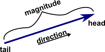
A vector is an essential concept in mathematics and physics. It’s like an arrow with a specific length (magnitude) and direction. Imagine a straight arrow in space. That arrow is a vector.

Components of a Vector:

• Magnitude: This is just a fancy word for the vector’s length or size. Imagine measuring the length of the arrow from its tail to its tip.
• Direction: Think of this as the way the arrow points. Does it go up, down, left, right, or at some angle?

In mathematical terms, we represent vectors using coordinates. For example:

• In 2D, a vector can be written as v = (x, y), where x and y represent the horizontal (x-axis) and vertical (y-axis) components, respectively.
• In 3D, vectors are represented as v = (x, y, z), incorporating a third dimension.
• And, in an N-dimensional space, a vector can be expressed as v = (x₁, x₂, x₃, …, xₙ), extending into multiple dimensions.

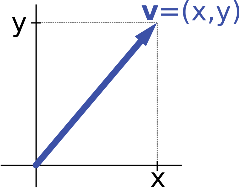
Vector Notation:

In most standard vector representations, the tail of the vector is considered as the origin (0, 0). This means that the coordinates of the vector’s endpoint are relative to the origin.

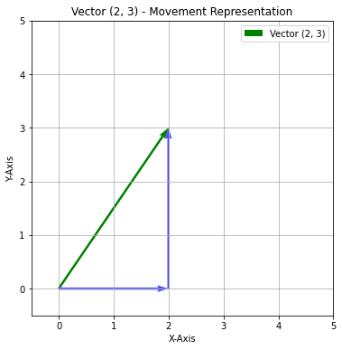
The coordinate (2, 3) in coordinate system is represented as:

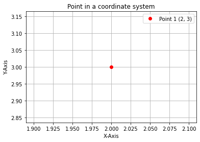
The above point (2, 3) in vector space will be represented by movement from origin. It means you move 2 units to the right (along the x-axis) and 3 units up (along the y-axis) from the origin (0, 0).

In the realm of technology and data science, vectors serve as the foundation for a wide range of applications, from computer graphics to machine learning.

For instance, in image processing, each pixel in a digital image can be represented as a vector of color values, allowing for complex operations like image manipulation and feature extraction.

Also, if we consider the world of natural language processing, text data, such as sentences or documents, can be represented as vectors using sophisticated techniques like word embeddings. These embeddings encode semantic meaning and context into numerical vectors, enabling computers to process and understand human language more effectively. Let’s understand them in more detail.

Word Embeddings

Imagine you have a big book filled with lots of words. Each word has its own unique meaning, and when we use these words in sentences, they help us communicate ideas and thoughts. Now, word embeddings are like a super-smart way of representing these words in a special numerical way that a computer can understand.

What are Word Embeddings?

At its core, a word embedding is a numerical representation of a word in a multi-dimensional space. Each word is mapped to a vector of real numbers, where the values in this vector encode semantic and syntactic information about the word. This transformation allows us to analyze and manipulate words using mathematical operations, opening up a wealth of possibilities for NLP tasks.

So, just as we humans know the context of the word “king” — where it is used and what it means — by representing words as word embeddings, machines also gain an understanding of the context of words. Therefore, we can say that machines can understand language with the help of word embeddings.

The word “king” can be represented as a vector of numbers, typically with a length of, for example, 150 dimensions. This vector might look something like this:

king=[0.1,0.05,0.2,…,150 numbers]

Each number in this vector carries specific information about the word “king” based on its usage and context in a large corpus of text.

The length of the vector (e.g., 150 dimensions) determines the level of detail and complexity in representing the word. More dimensions can potentially capture richer semantic information but require more computational resources.

How Do Word Embeddings Work?

To grasp the concept better, let’s visualize words as points in a high-dimensional space.

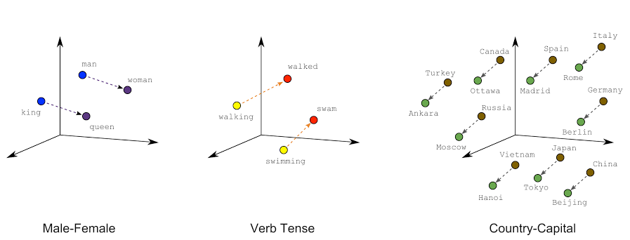
In the above image, we can see that the words that share similar contexts or meanings in language are positioned closer together in this space. For instance, words like “king” and “queen” would be located near each other because they often appear in similar contexts (royalty, monarchy, etc.).

For “walk” and “walking”, these words would be positioned closely together in the embedding space because they share a related meaning and often appear in similar contexts, representing the action of moving on foot. Similarly, “Canada” and “Ottawa” would be situated near each other in the embedding space due to their semantic relationship, reflecting that Ottawa is the capital city of Canada.

But this is not it. The magic lies in the mathematical relationships between these word vectors. By performing vector operations, such as addition or subtraction, we can uncover intriguing linguistic insights.

Imagine we have vectors representing words like “king,” “man,” “woman,” and “queen.” When we subtract the vector for “man” from “king” and then add the vector for “woman,” the resulting vector is very close to the vector for “queen.”

king - man + woman = queen

This ability to perform calculations with words helps computers grasp subtle meanings and relationships, making language processing more powerful and easy to understand.

Visualizing Word Embeddings

Let’s dive into the exciting world of word embeddings by visualizing them.

Setting up environment

We will be using OpenAIEmbeddings for our purpose. To use it, you will need an OpenAI API key.

Follow the below steps to generate OpenAI API Key:

1. First, create an OpenAI account or sign in.
2. Next, navigate to the API key page and “Create new secret key”, optionally naming the key. Make sure to save this somewhere safe and do not share it with anyone.

Once you have your key, we are ready to go.

import os
os.environ["OPENAI_API_KEY"] = "YOUR_API_KEY"

Step 2: Retrieving Embeddings

Let’s write a function that takes a word or sentence as an input and returns its embeddings.

from openai import OpenAI
 
client = OpenAI()
 
def get_openai_embedding(text, model="text-embedding-ada-002"):
    text = text.replace("\n", " ")
    return client.embeddings.create(input = [text], model=model).data[0].embedding

We are using “text-embedding-ada-002” model for Embeddings. You can check out more embedding models from OpenAI at OpenAI Embeddings models.

Step 3: Understanding Embeddings

Let’s see how word embeddings look like by retrieving the embedding for the word “queen”:

queen = get_openai_embedding("queen")
print("Length of queen", len(queen))
print(queen)

The output looks like:

The resulting embedding is a vector representation of the word “queen” in a high-dimensional space (1536 dimensions for text-embedding-ada-002).

Step 4: Writing function to visualize words

The retrieved embeddings are high-dimensional (e.g., 1536 dimensions), making it challenging to directly visualize them. Hence, we use PCA (Principal Component Analysis) to reduce the dimensionality to 2D for visualization purposes.

Let’s start with importing necessary libraries.

import matplotlib.pyplot as plt
from sklearn.decomposition import PCA 

Now, define a function to visualize word embeddings in 2D space:

def visualize_pca_2d(embeddings, words):
    pca_2d = PCA(n_components=2)
    embeddings_2d = pca_2d.fit_transform(embeddings)

    # Create a 2D scatter plot
    plt.figure(figsize=(10, 6))
    plt.scatter(embeddings_2d[:, 0], embeddings_2d[:, 1], marker='o')
    for i, word in enumerate(words):
        plt.annotate(word, (embeddings_2d[i, 0], embeddings_2d[i, 1]))

    plt.xlabel("Principal Component 1")
    plt.ylabel("Principal Component 2")
    plt.title("2D Visualization of Word Embeddings")
    plt.grid(True)
    plt.show()

Now, let’s visualize embeddings for a list of words:

words = ['cat', 'dog', 'bike', 'kitten', 'puppy', 'bicycle', 'aeroplane', 'helicopter', 'cow', 'wolf', 'lion', 'fighter jet']
embeddings = []
for i in words:
    embeddings.append(get_openai_embedding(i))
visualize_pca_2d(embeddings, words)

We get the plot as:

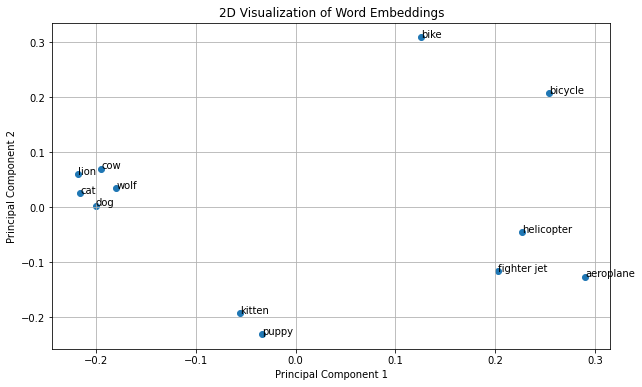
In the above plot, we observe meaningful clusters that reflect semantic relationships between words. Animal-related terms like “lion,” “cow,” “cat,” “dog,” and “wolf” form a distinct group due to their shared semantic context. Similarly, air transportation-related words such as “aeroplane,” “helicopter,” and “fighter jet” cluster together, indicating common associations related to transportation. Additionally, pet names like “kitten” and “puppy” are closely grouped, highlighting their shared attributes as young animals. Interestingly, the transportation cluster appears closer to each other compared to the animal cluster, suggesting stronger semantic relationships within this category.

Feel free to explore more word combinations and share your observations in the comments below!

Pythagorean Theorem

Remember our school friend from maths, Pythagoras? Well, he gifted us a marvelous discovery known as the Pythagorean Theorem. This fundamental theorem holds the key to understanding the relationships within right-angled triangles. Let’s delve into the magic of right triangles and how this theorem works its wonders!

Understanding the Pythagorean Theorem

In a right-angled triangle, the Pythagorean Theorem states that the square of the length of the hypotenuse (the side opposite the right angle) is equal to the sum of the squares of the lengths of the other two sides.

Mathematically, for a right triangle with sides of lengths ‘a’ and ‘b’, and a hypotenuse of length ‘c’, the Pythagorean Theorem can be expressed as:

c2 = a2 + b2

Let’s bring this theorem to life with a practical example and a visual diagram.

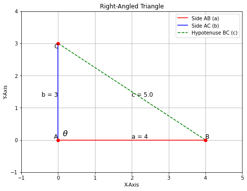
In the above plot, we can see that we have three sides, with c = 5 units, a = 4 units and b = 3 units.

Now, let’s prove the Pythagorean Theorem using our example: c² = a² + b²

c2 = a2 + b2
52 = 42 + 32
25 = 16 + 9
25 = 25

Voila! The theorem holds true, showcasing the beautiful symmetry and relationship between the sides of a right triangle.

Extending the Pythagorean Theorem: Calculating Distance in 2D Space

Let’s dive in and follow along with the code in your notebook!

Step 1: Two Points – Define the Points

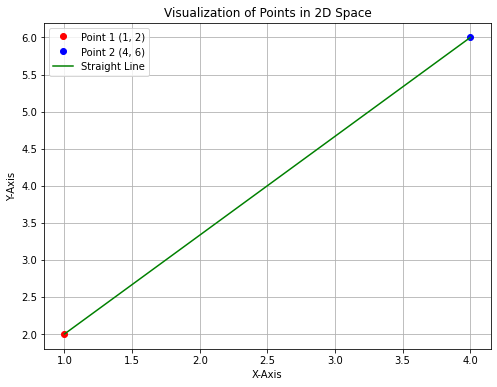
Imagine two points in a 2-D space. These points can represent anything from physical locations to abstract quantities.

point1 = (1, 2)
point2 = (4, 6)

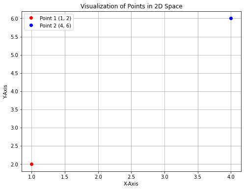
Step 2: Connecting a Line – Calculate Differences and Hypotenuse

To measure the distance between these points, connect them with a straight line. This line represents the shortest path between the two points, equivalent to the hypotenuse of a right-angled triangle.

Step 3: Calculate the differences in coordinates

To measure the distance between two points in a 2-dimensional space, we start by calculating the differences in their x-coordinates (horizontal) and y-coordinates (vertical).

side1 = point2[0] - point1[0]
side2 = point2[1] - point1[1]
print(f"Length of side1 is {side1} units")
print(f"Length of side2 is {side2} units")

We get the output as:

Length of side1 is 3 units
Length of side2 is 4 units

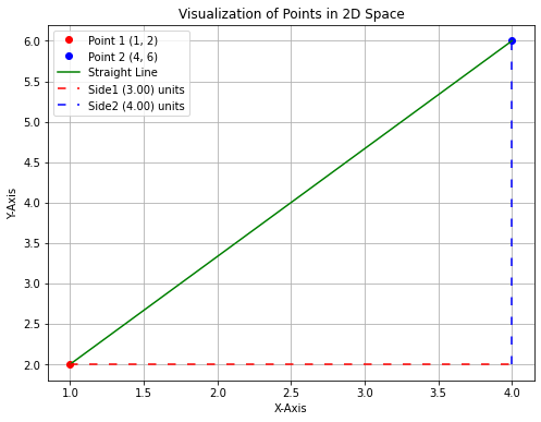
As observed in the plot above, it resembles a right-angled triangle, where the straight line connecting the two points acts as the hypotenuse, and the calculated differences (side1 and side2) represent the lengths of the other two sides. We’ve already computed the lengths of these sides.

Now, let’s apply the Pythagorean Theorem to calculate the length of the hypotenuse, which will determine the distance between these two points.

hypotenuse_square = side1**2 + side2**2
distance_2d = math.sqrt(hypotenuse_square)
print(f"The length of the hypotenuse, i.e., distance between two points is {distance_2d} units")

The output of the above code is:

The length of the hypotenuse, i.e., distance between two points is 5.0 units

So for two dimension, we can also represent the distance as:

distance_2d = ((point2[0] - point1[0])**2 + (point2[1] -point1[1])**2)**0.5
print("Distance between 2D points:", distance_2d)

The output for the above code is:

Distance between 2D points: 5.0 

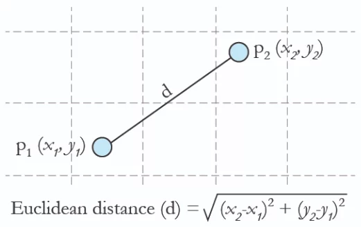
Step 4: Deriving Euclidean Distance

Now, let’s represent the coordinates in terms of x and y:-

point1 = (1, 2)
point2 = (4, 6)
\({x_2}\) = point2[0] = 4
\({x_1}\) = point1[0] = 1
\({y_2}\) = point2[1] = 6
\({y_1}\) = point1[1] = 2
distance = \(\sqrt{(x_2 – x_1)^2 + (y_2 – y_1)^2}\)
distance = \(\sqrt{(4 – 1)^2 + (6 – 2)^2}\)
distance = \(\sqrt{9 + 16}\)
distance = \(\sqrt{25}\)
distance = 5

This is called euclidean distance.

Extending the Pythagorean theorem to 3-dimension

Now, let’s extend this idea into three dimensions, where distances involve not only length and width but also height.

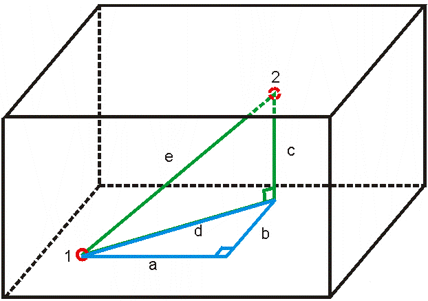
In the above figure, distance ‘e’ would be the distance between point 1 & point 2. We could determine it using Pythagorean theorem as seen previously, but we first need to find the value of ‘d’ using values ‘a’ and ‘b’.

Using Pythagorean theorem, we know that for triangle ABD,

d2 = a2 + b2

And for triangle ECD,

e2 = d2 + c2

If we substitute the value of d² in this equation, it becomes:

e2 = a2 + b2 + c2

e = \(\sqrt{a^2+b^2 + c^2}\)

So, now we can use this formula to calculate the length of ‘e’. Let’s do it.

Step 1: Define two Points in 3D

point1 = (1, 2, 3)
point2 = (4, 6, 8)

Step 2: Calculate the differences in coordinates

delta_x = point2[0] - point1[0]
delta_y = point2[1] - point1[1]
delta_z = point2[2] - point1[2]

distance_3d = (delta_x**2 + delta_y**2 + delta_z**2)**0.5
print("Distance between 3D points:", distance_3d)

The output for the above code is:

Distance between 3D points: 7.0710678118654755 

So we are able to calculate distance between two points in 3 dimension. Again, we can represent the distance as:

point1 = (1, 2, 3)
point2 = (4, 6, 8)
distance = hypotenuse
distance = \(\sqrt{hypotenuse^2}\)
distance = \(\sqrt{\Delta x^2 + \Delta y^2 + \Delta z^2}\)
distance = \(\sqrt{(point2[0] – point1[0])^2 + (point2[1] – point1[1])^2 + (point2[2] – point1[2])^2}\)

In code, it looks like:

distance_3d = ((point2[0] - point1[0])**2 + (point2[1] - point1[1])**2 + (point2[2] - point1[2])**2)**0.5

print("Distance between 3D points:", distance_3d)

The output for the above code is:

Distance between 3D points: 7.0710678118654755 

So euclidean distance for 3-D becomes as:

distance = \(\sqrt{(x_2 – x_1)^2 + (y_2 – y_1)^2 + (z_2 – z_1)^2}\)

Extending the Pythagorean theorem to n-dimension

# Calculate the Euclidean distance
def calculate_distance(point1, point2):
    distance_nd = sum((x - y) ** 2 for x, y in zip(point2, point1))**0.5
    return distance_nd

Let’s create two coordinates in 6 dimension.

point1 = (1, 2, 3, 4, 7, 4)
point2 = (4, 6, 8, 10, 8, 6)
calculate_distance(point1, point2)

The output of the above code is:

9.539392014169456

So, Euclidean distance for n-d becomes as

distance = \(\sqrt{(x_2 – x_1)^2 + (y_2 – y_1)^2 + (z_2 – z_1)^2 + (a_2 – a_1)^2 + …………}\)

where x, y, z, a ….., each represent a dimension/axis.

Or we can say that, for two points p and q in n-dimension,

d(p, q) = \(\sqrt{(q_1 – p_1)^2 + (q_2 – p_2)^2 + (q_3 – p_3)^2 + (q_4 – p_4)^2 + …………}\)

which comes as,

distance = \(\sqrt{\sum_{i=1}^{n} (q_i – p_i)^2 }\)

where ‘i’ represents a dimension and ‘n’ total number of dimensions.

Now, we can use this formula to calculate the distance between two embeddings, as they are N-dimensional vectors. As we know, the closer two embeddings are, the more similar they are.

Calculating distance between two embeddings

First, let’s compute the embeddings of four words.

cat = get_openai_embedding('cat')
dog = get_openai_embedding('dog')
car = get_openai_embedding('car')
bike = get_openai_embedding('bike')

Let’s use the calculate_distance() function to compute distances between various word embeddings:

distance_cat_dog = calculate_distance(cat, dog)
distance_cat_car = calculate_distance(cat, car)
distance_cat_bike = calculate_distance(cat, bike)
distance_bike_car = calculate_distance(bike, car)
distance_bike_dog = calculate_distance(bike, dog)

Now, let’s see how the distance looks like between these embeddings:

print(f"Distance between 'cat' and 'dog': {distance_cat_dog:.2f}")
print(f"Distance between 'cat' and 'car': {distance_cat_car:.2f}")
print(f"Distance between 'cat' and 'bike': {distance_cat_bike:.2f}")
print(f"Distance between 'bike' and 'car': {distance_bike_car:.2f}")
print(f"Distance between 'bike' and 'dog': {distance_bike_dog:.2f}")

The output of the above code is:

Distance between 'cat' and 'dog': 0.52
Distance between 'cat' and 'car': 0.56
Distance between 'cat' and 'bike': 0.61
Distance between 'bike' and 'car': 0.54
Distance between 'bike' and 'dog': 0.57

We can see, that ‘cat’ is closer to ‘dog’ than to ‘car’ or ‘bike’. Also, ‘bike’ is closer to ‘car’ than to ‘dog’ or ‘cat’. That means, the function is working fine.

Sentiment Analysis

In sentiment analysis, we want to understand whether a text expresses positive or negative feelings. Here’s a simple way to do it using word embeddings and basic geometry:

What We Do:

1. Choose Sentiment Words: We pick specific words that clearly indicate positive or negative sentiments, like ‘positive’ and ‘negative’. For each of these words, we get their embeddings.
   • Positive Sentiment: We find the embedding for the word ‘positive’ (embd_positive).
   • Negative Sentiment: Similarly, we find the embedding for ‘negative’ (embd_neg).
2. Calculate Distance: Now, when we have a review we want to analyze, we also get its embedding. We then calculate the distance between the review’s embedding and the embeddings of our sentiment words (embd_positive and embd_neg).
3. Make a Decision: Based on these distances:
   • If the review’s embedding is closer to embd_positive than to embd_neg, we say it’s a positive review.
   • Otherwise, if it’s closer to embd_neg, we say it’s negative.

Seems confusing? Let’s understand it with hands-on.

First, we start by obtaining embeddings for key sentiment words—’positive’ and ‘negative’:

embd_positive = get_openai_embedding('positive')
embd_neg = get_openai_embedding('negative')

Next, we calculate embeddings for two straightforward reviews:

embeddings_good_review = get_openai_embedding('The product is amazing')
embeddings_bad_review = get_openai_embedding('The product is not good')

Now, let’s use visualize_pca_2d() from before to visualize them.

sent_embeddings = np.array([embeddings_good_review, embeddings_bad_review, embd_positive, embd_neg])
visualize_pca_2d(sent_embeddings, words = ['The product is amazing', 'The product is not good','positive', 'negative'])

The above code outputs:

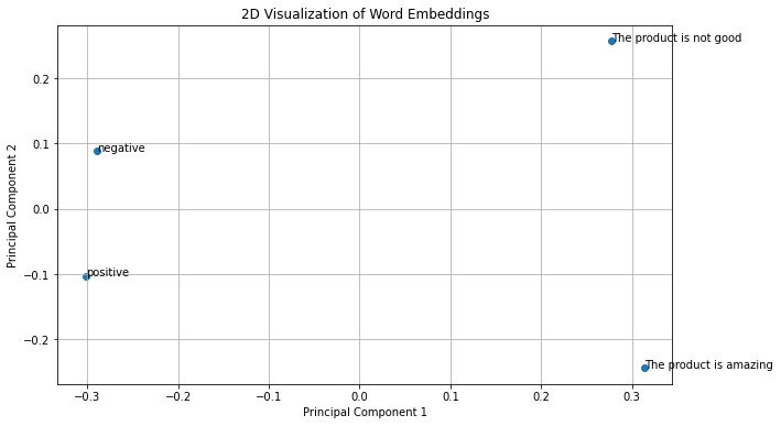
We can clearly see that embedding of ‘The product is amazing’ is closer to embedding of word ‘positive’ than the embedding of word “negative”. This shows that our approach works.

Now, armed with these embeddings, we can create a simple function sentiment(review) to classify reviews as positive or negative based on their proximity to our sentiment embeddings:

def sentiment(review):
    embed_review = get_openai_embedding(review)
    dist_pos = calculate_distance(embed_review, embd_positive)
    dist_neg = calculate_distance(embed_review, embd_neg)
    if dist_pos < dist_neg:
        print("It is a positive review")
        return True
    else:
        print("It is a negative review")
        return False

Let’s put our sentiment() function to the test with more complex reviews:

sentiment("Camera quality is too worst. Don't buy this if you want good photos. We can get this quality pictures with 5000 rupees android phone. I am totally disappointed because I expected range of iPhone camera quality but not this.. Waste of money.")

The output of the above code is:

It is a negative review

sentiment(""Worth to buy it. If you are managed money buy then buy it it never feels you waste of money. Performance. Hand in feel. Camera quality at flagship level"")

The output of the above code is:

It is a positive review 

Let’s try out more tricky reviews.

sentiment("At first it seemed like a great product but my expectations were changed completed.")

The output of the above code is:

It is a negative review

sentiment("At first, it seemed like a bad product but it met my expectations.")

The output of the above code is:

It is a positive review

Our sentiment() function demonstrates a straightforward yet effective approach to sentiment analysis using word embeddings. By leveraging pre-trained embeddings and simple distance calculations, we can accurately classify reviews based on their underlying sentiment. Feel free to experiment with different reviews and observe how the function performs in classifying sentiments!

Dot product between two vectors

Till now, we’ve been using Euclidean distance to measure similarity between vectors. However, another powerful method for gauging similarity is through the dot product.

The dot product, also known as the scalar product, is a way to measure how much two vectors are aligned or point in the same direction. Imagine vectors as arrows in space, and the dot product tells us how much one arrow overlaps with another.

Mathematically, the dot product of two vectors A and B is represented as A · B and is calculated as follows:

A = (A1, A2, A3, ……, An)

B = (B1, B2, B3, ……, Bn

A · B = A1 * B1 + A2 * B2 + A3 * B3 + … + An * Bn

So suppose two vectors are

A = (1,2,3)

B = (4,5,6)

A.B = (A[0] * B[0]) + (A[1] * B[1]) + (A[2] * B[2])

A.B = (1 * 4) + (2 * 5) + (3 * 6)

A.B = 32

What the Dot Product Represents?

The dot product gives us a number that represents how similar or aligned two vectors are. If the dot product is large, it means the vectors are pointing in similar directions. If it’s small, the vectors are more perpendicular or point in different directions.

Let’s understand it with the help of visualization.

Consider two vectors as:

A = (2,3)

B = (4,2)

So, if we plot them, they will look like:

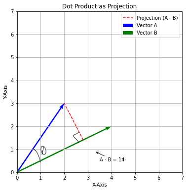
Imagine walking from the tail of vector A (2, 3) in the direction of vector B (4, 2) until you hit the line containing vector B. This imaginary path is the projection of A onto B (represented by dotted red line). The length of this projection (which is a dotted line segment in the image) is what matters for the dot product calculation.

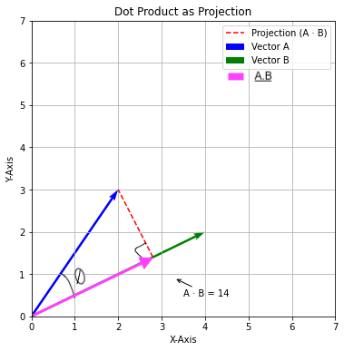
So, A.B will look like:

Applying Dot Product to Sentiment Analysis

Now, let’s leverage the dot product for sentiment analysis. Everything remains same. Just instead of using Euclidean Distance, we will be using dot product.

def sentiment_using_dot_product(review):
    embed_review = get_openai_embedding(review)
    dist_pos = np.dot(embed_review, embd_positive)
    dist_neg = np.dot(embed_review, embd_neg)
    if dist_pos > dist_neg:
        print("It is a positive review")
        return True
    else:
        print("It is a negative review")
        return False

Let’s try in Hindi language to see if it works.

is_positive2("ye product kaafi achha hai")

The output is:

It is a positive review

Let’s try for a negative review.

is_positive2("ye product kaafi kharaab hai")

The output is:

It is a negative review

So, that’s the benefit of using LLM Embeddings. It can understand sentiments in different languages.

Cosine Similarity

The dot product of two vectors measures their similarity in terms of both direction and magnitude. However, the dot product itself lacks a bounded range, making it less intuitive as a direct similarity metric. To address this limitation, we can use cosine similarity, which is a normalized version of the dot product.

Now let’s consider the plot from before, which is

In trigonometry, we have studied that: cos(θ) = adjacent side / hypotenuse

In the context of the dot product, the adjacent side is (A · B), and the hypotenuse is (|A| * |B|). Therefore, we have:

That makes cos θ = (A · B) / (|A| * |B|)

This is called as cosine similarity, another similarity measure for vectors. So, here we basically normalize the dot product by dividing it by the product of the magnitudes (or norms) of the vectors. The resulting similarity score ranges between -1 (perfectly opposite directions) and 1 (perfectly aligned directions). That makes cosine similarity more interpretable and suitable for various similarity measurement tasks.

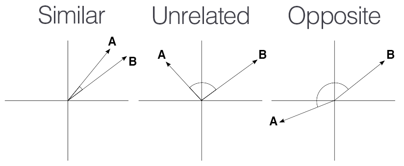
If the vectors are exactly the same, the cosine similarity is 1 (cos 0° = 1).

If the vectors are orthogonal (perpendicular), the cosine similarity is 0 (cos 90° = 0).

If the vectors are in opposite directions, the cosine similarity is -1 (cos 180° = -1).

Values in between indicate different degrees of similarity.

Let’s code it:

def cosine_similarity(A, B):
    dot_product = np.dot(A, B)

    # Calculate the magnitudes |A| and |B|
    magnitude_A = np.linalg.norm(A)
    magnitude_B = np.linalg.norm(B)

    # Calculate the cosine similarity
    cosine_similarity = dot_product / (magnitude_A * magnitude_B)
    return cosine_similarity

Now it’s homework for you to perform sentiment analysis using cosine similarity as the similarity measure.

Conclusion

Embarking on this journey into sentiment analysis with word embeddings has not only provided practical insights but has also highlighted the elegance and simplicity of leveraging embeddings for natural language understanding.

As you continue to explore the world of embeddings and NLP, remember that the applications extend far beyond sentiment analysis. From machine translation to text summarization and beyond, embeddings serve as foundational tools that underpin many advanced techniques in the field of natural language processing.

We encourage you to experiment further, refine your understanding, and delve deeper into the possibilities that embeddings offer. Whether you’re a seasoned practitioner or just beginning your NLP journey, the realm of word embeddings invites exploration and innovation.

Ready to take a deep dive into generative AI? Consider enrolling in our course, Hands-on Generative AI with Langchain and Python on CloudxLab. This course will equip you with the skills to build powerful generative models using Python and Langchain!