Fashion-MNIST using Machine Learning

One of the classic problem that has been used in the Machine Learning world for quite sometime is the MNIST problem. The objective is to identify the digit based on image. But MNIST is not very great problem because we come up with great accuracy even if we are looking at few pixels in the image. So, another common example problem against which we test algorithms is Fashion-MNIST.

The complete code for this project you can find here : https://github.com/cloudxlab/ml/tree/master/projects/Fashion-MNIST

Fashion-MNIST is a dataset of Zalando’s fashion article images —consisting of a training set of 60,000 examples and a test set of 10,000 examples. Each instance is a 28×28 grayscale image, associated with a label.

Objective

This work is part of my experiments with Fashion-MNIST dataset using various Machine Learning algorithms/models. The objective is to identify (predict) different fashion products from the given images using various best possible Machine Learning Models (Algorithms) and compare their results (performance measures/scores) to arrive at the best ML model. I have also experimented with ‘dimensionality reduction’ technique for this problem.

Acknowledgements

I have used Fashion-MNIST dataset for this experiment with Machine Learning. Fashion-MNIST dataset is a collection of fashion articles images provided by Zalando . Thanks to Zalando Research for hosting the dataset.

Understanding and Analysing the dataset

Fashion MNIST Training dataset consists of 60,000 images and each image has 784 features (i.e. 28×28 pixels). Each pixel is a value from 0 to 255, describing the pixel intensity. 0 for white and 255 for black.

The class labels for Fashion MNIST are:

Label	Description
0	T-shirt/top
1	Trouser
2	Pullover
3	Dress
4	Coat
5	Sandal
6	Shirt
7	Sneaker
8	Bag
9	Ankle boot

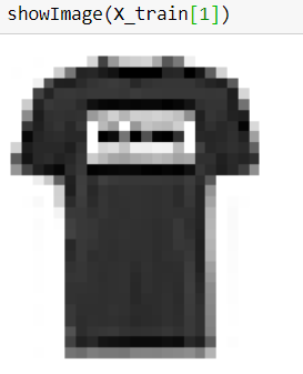
Let us have a look at one instance (an article image) of the training dataset.

Problem Definition

The ‘target’ dataset has 10 class labels, as we can see from above (0 – T-shirt/top, 1 – Trouser,,….9 – Ankle Boot).

Given the images of the articles, we need to classify them into one of these classes, hence, it is essentially a ‘Multi-class Classification’ problem.

We will be using various Classifiers and comparing their results/scores.

Preparing the Data

We already have the splitted dataset (training and test) available in ratio 85:15 (60,000:10,000) from Zalando Research, we will use the same for this experiment.

X_train, X_test, y_train, y_test = trainSet, testSet, trainLabel, testLabel

print(X_train.shape)
print(y_train.shape)
print(X_test.shape)
print(y_test.shape)

# Output
(60000, 784)
(60000,)
(10000, 784)
(10000,)

As part of data preparation, following techniques were applied on the dataset:

• • • Shuffling
    • Feature Scaling

We shuffle the training dataset to get uniform samples for cross-validation. This also  ensures that we don’t miss out any article in a cross-validation fold.

Each image (instance) in the dataset has 784 pixels (features) and value of each feature(pixel) ranges from 0 to 255, this range is too wide, hence we have performed feature scaling (using Standardization) on the training dataset, so that values of all features (pixels) are in a small range.

The scaled dataset is created using the below formula:

x_scaled = (x - x_mean) / standard deviation 

This essentially means that we calculate how many standard deviation away is each point from the mean.

Please note that scaling is not needed for Decision Tree based ML algorithms which also includes Random Forest and XGBoost.

Training various ML Models

Based on the problem type (multi-class classification), various relevant classifiers were used to train the model.

Training dataset was trained on following ML Algorithms:

1. 1. 1. SGD Classifier
      2. Softmax Regression
      3. Decision Tree Classifier
      4. Random Forest Classifier
      5. Ensemble with soft voting (with Softmax Regression and Random Forest Classifier)
      6. XGBoost Classifier

Since, accuracy score is not relevant for skewed dataset, and in future we may get skewed dataset, I decided to go for other scores too like – Precision, Recall, F1 score.

Validating the Training Results

During the training phase, I validated the results using k-fold cross-validation. Generally, 10 folds (cv=10) are used, but,  in this case, I used only 3 folds (cv=3), just to reduce the cross-validation time.

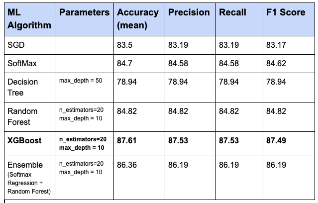
Below are the results for various ML models (algorithms) from cross-validation:

Standard deviation in all cases was around 0.0020, except for XGBoost (standard deviation – 0.00063).

Cross-validation was used to find the proper score of each model, and also to ensure that the model is not overfitting or underfitting.

From the cross-validation results above, we see that XGBoost model performs best in the training phase, hence, it was selected for the next steps of this problem.

Fine-Tuning the Selected Model

For fine-tuning of the selected XGBoost model, I used Grid Search technique.

Grid search process on training dataset (with 784 features) was taking a lot of time, hence I decided to go for Dimensionality Reduction (to get the reduced training dataset) to reduce the grid search and prediction time.

For dimensionality reduction, since it’s not Swiss-roll kind of data, I decided to go for PCA for this dataset.

I tried various values of variance ratio (0.95, 0.97, 0.99), but, since, 0.99 variance ratio gave enough number of features(459 features out of original 784 features) without losing any significant information (quality), I selected variance ratio of 0.99for performing the dimensionality reduction on the dataset.

Grid search was performed on the selected XGBoost model, on reduced training dataset with below set of hyperparameters:

n_estimators = [20]
max_depth=[8,10,12]

Below are the grid search results:

Best Parameters:

n_estimators = 20
max_depth = 10

Best Estimator – XGBClassifier with following parameter values:

learning_rate = 0.1
min_child_weight = 1
n_estimators=20
max_depth=10

Evaluating the Final Model on Test Dataset

I have used the final model, that we got from grid search (best estimator) above, for predictions on the reduced test dataset (got after applying dimensionality reduction with 0.99 variance ratio).

Following are the results for the test dataset:

Below are the Results from training dataset that we got earlier:

Conclusion

Difference between results (say accuracy score) of test dataset and training dataset is

As we see, the difference between scores of test dataset and training dataset is very low (3.3%), hence, the conclusion is that our final model (XGBoost) is good enough, and it doesn’t have any overfitting or underfitting.

Although XGBoost (with n_estimators=20 and max_depth = 10) is good enough, there may be a chance to improve this model further, by say, increasing the number of estimators and trying out some more hyperparameters.

As we see above, Ensemble also has given good results, we can try Ensemble with some more models and with some more hyperparameters to improve the results further.

This experiment was limited to Machine Learning algorithms. You can try Deep Learning techniques (say CNN, etc.) to improve the results further.

I didn’t try SVM for this problem, because for larger dataset, SVM (kernel=poly) takes a long time to train.

Again, for your reference, the complete code for this project you can find here : https://github.com/cloudxlab/ml/tree/master/projects/Fashion-MNIST

For the complete course on Machine Learning, please visit Specialization Course on Machine Learning & Deep Learning