Usually, the learners from our classes schedule 1-on-1 discussions with the mentors to clarify their doubts. So, thought of sharing the video of one of these 1-on-1 discussions that one of our CloudxLab learner – Leo – had with Sandeep last week.
Below are the questions from the same discussion.
You can go through the detailed discussion which happened around these questions, in the attached video below.
Q.1. In the Life Cycle of Node Value chapter, please explain me the below line of code. What are zz_v, z_v and y_v values ?
zz_v, z_v, y_v = s.run([zz, z, y] Ans.1. The complete code looks like below:
w = tf.constants(3)
x = w + 2
y = x + 5
z = x + 3
zz = tf.square(y+z)
with tf.Session() as s:
    zz_v, z_v, y_v = s.run([zz, z, y])
print(zz_y)
s.run([zz, z, y]) expression above is basically evaluating zz, z and y, and is returning their evaluated values, which we are storing in variables zz_v, z_v and y_v variables respectively. Basically, the the run function of session object returns the same data type as passed in the first argument. Here, the run method is returning an array of values.
TensorFlow is a Python library and in Python, we can return multiple values from a function in the form of a tuple. Here is a simple example:
x, y , z = [2, 3, 4]
print(x)
2
print(y)
3
print(z)
4
Same thing is happening here, s.run() is returning multiple values which are being stored in variables zz_v, z_v and y_v respectively.
So, the evaluated value of zz is stored in variable zz_v, evaluated value of variable z in z_v and evaluated value of variable y in variable y_z.
Q.2. In Linear Regression chapter, we are using housing price dataset. How do we know that the model for housing price dataset is a linear equation ? Is it just an assumption ?
Ans.2. Yes, it is an assumption that model for housing price dataset is a linear equation.
We can use linear equation for a non-linear problem also.
We convert most of the non-linear problems into a linear problem by using polynomial features.
Even Polynomial Regression problem is solved using Linear Regression by converting a non-linear problem to linear problem by adding polynomial features.
y = ϴ0 + ϴ1 x + ϴ2 x1 + ϴ3 x2 + ...Suppose your equation is
where x1 and x2 are polynomial features and
x1 = square(x)
x2 = cube(x)
ϴ0, ϴ1, ϴ2, …. etc are weights or also called coefficients.
In Linear Regression, when Gradient Descent is applied on this equation, weights ϴ1 and ϴ3 will go down to 0 (zero) and weight ϴ2 will become bigger. Hence, at the end of Gradient Descent, our above equation will look like below i.e. we get a non-linear equation
y = ϴ0 + ϴ2 x1
or , y = ϴ0 + ϴ2 square(x)
Q.3. Equations of Gradient and Gradient Descent, I don’t understand them
Ans.3.
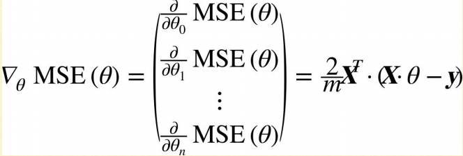
The below equation is for calculating the Gradient

MSE is ‘Mean Squared Error’
m is total number of instances.
X dataset is a matrix with ‘n’ columns (features) and ‘m’ rows (instances).
y is a vector (containing actual values of label) with ‘m’ rows and 1 column
y^ is a also a vector (containing predicted values of label) with ‘m’ rows and 1 column
y = ϴ0 + ϴ1 x1 + ϴ2 x2
MSE (E) = square(y∧ - y) / m
MSE (E) = square(ϴ0 + ϴ1 x1 + ϴ2 x2 - y) / m
∂(MSE)/∂ϴ0 = 2(ϴ0 + ϴ1 x1 + ϴ2 x2 - y) / m
               = 2/m (X.ϴ - y )
∂(MSE)/∂ϴ1 = 2(ϴ0 + ϴ1 x1 + ϴ2 x2 - y) x1 / m
               = 2/m (X.ϴ - y) X
               = 2/m X (X.ϴ - y)
Therefore, we get,
Below equation is for calculating the Gradient Descent

η is the learning rate here.
ϴ is an array of theta values.

is also an array of values, and is called the Gradient or the rate of change of error (E).
If the Gradient increases, we need to decrease the ϴ, and if the Gradient decreases, we need to increase the ϴ. Eventually, we need to move towards making the Gradient equal to 0 (zero) or nearly 0.
Q.4. In Gradient Descent, what we can do to avoid getting stuck in local minima ?
Ans.4. You can use Stochastic Gradient Descent to avoid getting stuck in local minima.
You can find more details about this in our Machine Learning course.
For the complete course on Machine Learning, please visit Specialization Course on Machine Learning & Deep Learning