Python is increasingly being used as a scientific language. Matrix and vector manipulations are extremely important for scientific computations. Both NumPy and Pandas have emerged to be essential libraries for any scientific computation, including machine learning, in python due to their intuitive syntax and high-performance matrix computation capabilities.
In this post, we will provide an overview of the common functionalities of NumPy and Pandas. We will realize the similarity of these libraries with existing toolboxes in R and MATLAB. This similarity and added flexibility have resulted in wide acceptance of python in the scientific community lately. Topic covered in the blog are:
- Overview of NumPy
- Overview of Pandas
- Using Matplotlib
This post is an excerpt from a live hands-on training conducted by CloudxLab on 25th Nov 2017. It was attended by more than 100 learners around the globe. The participants were from countries namely; United States, Canada, Australia, Indonesia, India, Thailand, Philippines, Malaysia, Macao, Japan, Hong Kong, Singapore, United Kingdom, Saudi Arabia, Nepal, & New Zealand.
What is NumPy?
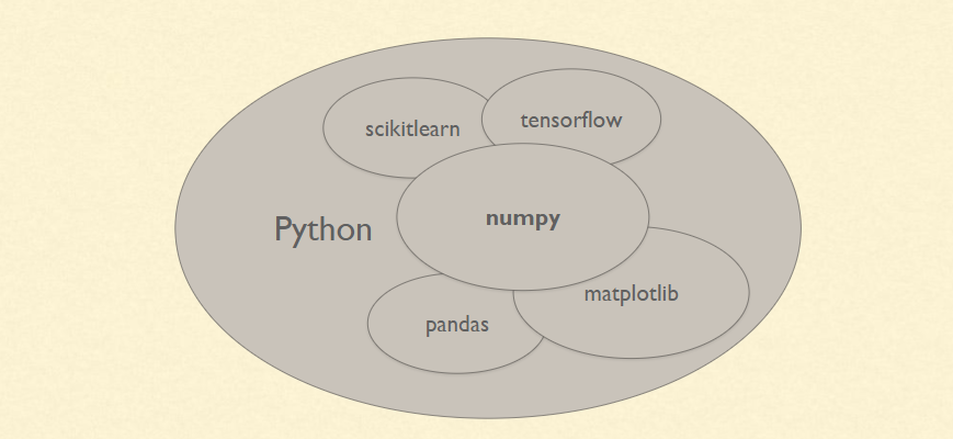
NumPy stands for ‘Numerical Python’ or ‘Numeric Python’. It is an open source module of Python which provides fast mathematical computation on arrays and matrices. Since, arrays and matrices are an essential part of the Machine Learning ecosystem, NumPy along with Machine Learning modules like Scikit-learn, Pandas, Matplotlib, TensorFlow, etc. complete the Python Machine Learning Ecosystem.
NumPy provides the essential multi-dimensional array-oriented computing functionalities designed for high-level mathematical functions and scientific computation. Numpy can be imported into the notebook using
>>> import numpy as np
NumPy’s main object is the homogeneous multidimensional array. It is a table with same type elements, i.e, integers or string or characters (homogeneous), usually integers. In NumPy, dimensions are called axes. The number of axes is called the rank.
There are several ways to create an array in NumPy like np.array, np.zeros, no.ones, etc. Each of them provides some flexibility.
| Command to create an array | Example |
| np.array |
>>> a = np.array([1, 2, 3]) >>> type(a) <type 'numpy.ndarray'> >>> b = np.array((3, 4, 5)) >>> type(b) <type 'numpy.ndarray'> |
| np.ones |
>>> np.ones( (3,4), dtype=np.int16 ) array([[ 1, 1, 1, 1], [ 1, 1, 1, 1], [ 1, 1, 1, 1]]) |
| np.full |
>>> np.full( (3,4), 0.11 ) array([[ 0.11, 0.11, 0.11, 0.11], [ 0.11, 0.11, 0.11, 0.11], [ 0.11, 0.11, 0.11, 0.11]]) |
| np.arange |
>>> np.arange( 10, 30, 5 ) array([10, 15, 20, 25]) >>> np.arange( 0, 2, 0.3 ) # it accepts float arguments array([ 0. , 0.3, 0.6, 0.9, 1.2, 1.5, 1.8]) |
| np.linspace |
>>> np.linspace(0, 5/3, 6) array([0. , 0.33333333 , 0.66666667 , 1. , 1.33333333 1.66666667]) |
| np.random.rand(2,3) |
>>> np.random.rand(2,3) array([[ 0.55365951, 0.60150511, 0.36113117], [ 0.5388662 , 0.06929014, 0.07908068]]) |
| np.empty((2,3)) |
>>> np.empty((2,3)) array([[ 0.21288689, 0.20662218, 0.78018623], [ 0.35294004, 0.07347101, 0.54552084]]) |
Some of the important attributes of a NumPy object are:
- Ndim: displays the dimension of the array
- Shape: returns a tuple of integers indicating the size of the array
- Size: returns the total number of elements in the NumPy array
- Dtype: returns the type of elements in the array, i.e., int64, character
- Itemsize: returns the size in bytes of each item
- Reshape: Reshapes the NumPy array
NumPy array elements can be accessed using indexing. Below are some of the useful examples:
- A[2:5] will print items 2 to 4. Index in NumPy arrays starts from 0
- A[2::2] will print items 2 to end skipping 2 items
- A[::-1] will print the array in the reverse order
- A[1:] will print from row 1 to end
The session covers these and some important attributes of the NumPy array object in detail.
Vectors and Machine learning
Machine learning uses vectors. Vectors are one-dimensional arrays. It can be represented either as a row or as a column array.
What are vectors? Vector quantity is the one which is defined by a magnitude and a direction. For example, force is a vector quantity. It is defined by the magnitude of force as well as a direction. It can be represented as an array [a,b] of 2 numbers = [2,180] where ‘a’ may represent the magnitude of 2 Newton and 180 (‘b’) represents the angle in degrees.
Another example, say a rocket is going up at a slight angle: it has a vertical speed of 5,000 m/s, and also a slight speed towards the East at 10 m/s, and a slight speed towards the North at 50 m/s. The rocket’s velocity may be represented by the following vector: [10, 50, 5000] which represents the speed in each of x, y, and z-direction.
Similarly, vectors have several usages in Machine Learning, most notably to represent observations and predictions.
For example, say we built a Machine Learning system to classify videos into 3 categories (good, spam, clickbait) based on what we know about them. For each video, we would have a vector representing what we know about it, such as: [10.5, 5.2, 3.25, 7.0]. This vector could represent a video that lasts 10.5 minutes, but only 5.2% viewers watch for more than a minute, it gets 3.25 views per day on average, and it was flagged 7 times as spam.
As you can see, each axis may have a different meaning. Based on this vector, our Machine Learning system may predict that there is an 80% probability that it is a spam video, 18% that it is clickbait, and 2% that it is a good video. This could be represented as the following vector: class_probabilities = [0.8,0.18,0.02].
As can be observed, vectors can be used in Machine Learning to define observations and predictions. The properties representing the video, i.e., duration, percentage of viewers watching for more than a minute are called features.
Since the majority of the time of building machine learning models would be spent in data processing, it is important to be familiar to the libraries that can help in processing such data.
Why NumPy and Pandas over regular Python arrays?
In python, a vector can be represented in many ways, the simplest being a regular python list of numbers. Since Machine Learning requires lots of scientific calculations, it is much better to use NumPy’s ndarray, which provides a lot of convenient and optimized implementations of essential mathematical operations on vectors.
Vectorized operations perform faster than matrix manipulation operations performed using loops in python. For example, to carry out a 100 * 100 matrix multiplication, vector operations using NumPy are two orders of magnitude faster than performing it using loops.
Some ways in which NumPy arrays are different from normal Python arrays are:
- If you assign a single value to a ndarray slice, it is copied across the whole slice
| NumPy Array | Regular Python array |
>>> a = np.array([1, 2, 5, 7, 8]) >>> a[1:3] = -1 >>> a array([ 1, -1, -1, 7, 8]) |
>>> b = [1, 2, 5, 7, 8] >>> b[1:3] = -1 TypeError: can only assign an iterable |
So, it is easier to assign values to a slice of an array in a NumPy array as compared to a normal array wherein it may have to be done using loops.
- ndarray slices are actually views on the same data buffer. If you modify it, it is going to modify the original ndarray as well.
| NumPy array slice | Regular python array slice |
>>> a = np.array([1, 2, 5, 7, 8]) >>> a_slice = a[1:5] >>> a_slice[1] = 1000 >>> a array([ 1, 2, 1000, 7, 8]) # Original array was modified |
>>> a=[1,2,5,7,8]
>>> b=a[1:5]
>>> b[1]=3
>>> print(a)
>>> print(b)
[1, 2, 5, 7, 8]
[2, 3, 7, 8]
|
If we need a copy of the NumPy array, we need to use the copy method as another_slice = another_slice = a[2:6].copy(). If we modify another_slice, a remains same
- The way multidimensional arrays are accessed using NumPy is different from how they are accessed in normal python arrays. The generic format in NumPy multi-dimensional arrays is:
Array[row_start_index:row_end_index, column_start_index: column_end_index]
NumPy arrays can also be accessed using boolean indexing. For example,
>>> a = np.arange(12).reshape(3, 4)
array([[ 0, 1, 2, 3], [ 4, 5, 6, 7], [ 8, 9, 10, 11]])
>>> rows_on = np.array([True, False, True])
>>> a[rows_on , : ]      # Rows 0 and 2, all columns
array([[ 0,  1,  2,  3],
      [ 8,  9, 10, 11]])
NumPy arrays are capable of performing all basic operations such as addition, subtraction, element-wise product, matrix dot product, element-wise division, element-wise modulo, element-wise exponents and conditional operations.
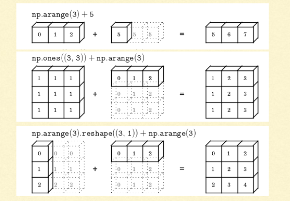
An important feature with NumPy arrays is broadcasting.

In general, when NumPy expects arrays of the same shape but finds that this is not the case, it applies the so-called broadcasting rules.
Basically, there are 2 rules of Broadcasting to remember:
- For the arrays that do not have the same rank, then a 1 will be prepended to the smaller ranking arrays until their ranks match. For example, when adding arrays A and B of sizes (3,3) and (,3) [rank 2 and rank 1], 1 will be prepended to the dimension of array B to make it (1,3) [rank=2]. The two sets are compatible when their dimensions are equal or either one of the dimension is 1.
- When either of the dimensions compared is one, the other is used. In other words, dimensions with size 1 are stretched or “copied” to match the other. For example, upon adding a 2D array A of shape (3,3) to a 2D ndarray B of shape (1, 3). NumPy will apply the above rule of broadcasting. It shall stretch the array B and replicate the first row 3 times to make array B of dimensions (3,3) and perform the operation.
NumPy provides basic mathematical and statistical functions like mean, min, max, sum, prod, std, var, summation across different axes, transposing of a matrix, etc.
A particular NumPy feature of interest is solving a system of linear equations. NumPy has a function to solve linear equations. For example,
2x + 6y = 6
5x + 3y = -9
Can be solved in NumPy using
>>> coeffs  = np.array([[2, 6], [5, 3]])
>>> depvars = np.array([6, -9])
>>> solution = linalg.solve(coeffs, depvars)
>>> solution
array([-3.,  2.])
What is Pandas?
Similar to NumPy, Pandas is one of the most widely used python libraries in data science. It provides high-performance, easy to use structures and data analysis tools. Unlike NumPy library which provides objects for multi-dimensional arrays, Pandas provides in-memory 2d table object called Dataframe. It is like a spreadsheet with column names and row labels.
Hence, with 2d tables, pandas is capable of providing many additional functionalities like creating pivot tables, computing columns based on other columns and plotting graphs. Pandas can be imported into Python using:
>>> import pandas as pd
Some commonly used data structures in pandas are:
- Series objects: 1D array, similar to a column in a spreadsheet
- DataFrame objects: 2D table, similar to a spreadsheet
- Panel objects: Dictionary of DataFrames, similar to sheet in MS Excel
Pandas Series object is created using pd.Series function. Each row is provided with an index and by defaults is assigned numerical values starting from 0. Like NumPy, Pandas also provide the basic mathematical functionalities like addition, subtraction and conditional operations and broadcasting.
Pandas dataframe object represents a spreadsheet with cell values, column names, and row index labels. Dataframe can be visualized as dictionaries of Series. Dataframe rows and columns are simple and intuitive to access. Pandas also provide SQL-like functionality to filter, sort rows based on conditions. For example,
>>> people_dict = { "weight": pd.Series([68, 83, 112],index=["alice", "bob", "charles"]),   "birthyear": pd.Series([1984, 1985, 1992], index=["bob", "alice", "charles"], name="year"),
"children": pd.Series([0, 3], index=["charles", "bob"]),
"hobby": pd.Series(["Biking", "Dancing"], index=["alice", "bob"]),}
>>> people = pd.DataFrame(people_dict)
>>> people

>>> people[people["birthyear"] < 1990]

New columns and rows can be easily added to the dataframe. In addition to the basic functionalities, pandas dataframe can be sorted by a particular column.
Dataframes can also be easily exported and imported from CSV, Excel, JSON, HTML and SQL database. Some other essential methods that are present in dataframes are:
- head(): returns the top 5 rows in the dataframe object
- tail(): returns the bottom 5 rows in the dataframe
- info(): prints the summary of the dataframe
- describe(): gives a nice overview of the main aggregated values over each column
What is matplotlib?
Matplotlib is a 2d plotting library which produces publication quality figures in a variety of hardcopy formats and interactive environments. Matplotlib can be used in Python scripts, Python and IPython shell, Jupyter Notebook, web application servers and GUI toolkits.
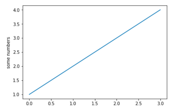
matplotlib.pyplot is a collection of functions that make matplotlib work like MATLAB. Majority of plotting commands in pyplot have MATLAB analogs with similar arguments. Let us take a couple of examples:
| Example 1: Plotting a line graph | Example 2: Plotting a histogram |
>>> import matplotlib.pyplot as plt
>>> plt.plot([1,2,3,4])
>>> plt.ylabel('some numbers')
>>> plt.show()
|
>>> import matplotlib.pyplot as plt
>>> x = [21,22,23,4,5,6,77,8,9,10,31,32,33,34,35,36,37,18,49,50,100]
>>> num_bins = 5
>>> plt.hist(x, num_bins, facecolor='blue')
>>> plt.show()
|


