1. Introduction
In this data analytics case study, we will use the US census data to build a model to predict if the income of any individual in the US is greater than or less than USD 50000 based on the information available about that individual in the census data.
The dataset used for the analysis is an extraction from the 1994 census data by Barry Becker and donated to the public site http://archive.ics.uci.edu/ml/datasets/Census+Income. This dataset is popularly called the “Adult” data set. The way that we will go about this case study is in the following order:
- Describe the data- Specifically the predictor variables (also called independent variables features) from the Census data and the dependent variable which is the level of income (either “greater than USD 50000” or “less than USD 50000”).
- Acquire and Read the data- Downloading the data directly from the source and reading it.
- Clean the data- Any data from the real world is always messy and noisy. The data needs to be reshaped in order to aid exploration of the data and modeling to predict the income level.
- Explore the independent variables of the data- A very crucial step before modeling is the exploration of the independent variables. Exploration provides great insights to an analyst on the predicting power of the variable. An analyst looks at the distribution of the variable, how variable it is to predict the income level, what skews it has, etc. In most analytics project, the analyst goes back to either get more data or better context or clarity from his finding.
- Build the prediction model with the training data- Since data like the Census data can have many weak predictors, for this particular case study I have chosen the non-parametric predicting algorithm of Boosting. Boosting is a classification algorithm (here we classify if an individual’s income is “greater than USD 50000” or “less than USD 50000”) that gives the best prediction accuracy for weak predictors. Cross validation, a mechanism to reduce over fitting while modeling, is also used with Boosting.
- Validate the prediction model with the testing data- Here the built model is applied on test data that the model has never seen. This is performed to determine the accuracy of the model in the field when it would be deployed. Since this is a case study, only the crucial steps are retained to keep the content concise and readable.
2. About the Data
As mentioned earlier, the data set is from http://archive.ics.uci.edu/ml/datasets/Census+Income.
2.1 Dependent Variable
The dependent variable is “incomelevel”, representing the level of income. A value of “<=50K” indicates “less than or equal to USD 50000” and “>50K” indicates “greater than USD 50000”.
2.2 Independent Variable
Below are the independent variables (features or predictors) from the Census Data
| Variable Name | Description | Type | Possible Values |
|---|---|---|---|
| Age | Age of the individual | Continuous | Numeric |
| Workclass | Class of Work | Categorical | Private, Self-emp-not-inc, Self-emp-inc, Federal-gov, Local-gov, State-gov, Without-pay, Never-worked |
| fnlwgt | Final Weight Determined by Census Org | Continuous | Numeric |
| Education | Education of the individual | Ordered Factor | Bachelors, Some-college, 11th, HS-grad, Prof-school, Assoc-acdm, Assoc-voc, 9th, 7th-8th, 12th, Masters, 1st-4th, 10th, Doctorate, 5th-6th, Preschool |
| Education-num | Number of years of education | Continuous | Numeric |
| Marital-status | Marital status of the individual | Categorical | Married-civ-spouse, Divorced, Never-married, Separated, Widowed, Married-spouse-absent, Married-AF-spouse |
| Occupation | Occupation of the individual | Categorical | Tech-support, Craft-repair, Other-service, Sales, Exec-managerial, Prof-specialty, Handlers-cleaners, Machine-op-inspct, Adm-clerical, Farming-fishing, Transport-moving, Priv-house-serv, Protective-serv, Armed-Forces |
| Relationship | Present relationship | Categorical | Wife, Own-child, Husband, Not-in-family, Other-relative, Unmarried |
| Race | Race of the individual | Categorical | White, Asian-Pac-Islander, Amer-Indian-Eskimo, Other, Black |
| Sex | Sex of the individual | Categorical | Female, Male |
| Capital-gain | Capital gain made by the individual | Continuous | Numeric |
| Capital-loss | Capital loss made by the individual | Continuous | Numeric |
| Hours-per-week | Average number of hours spent by the individual on work | Continuous | Numeric |
| Native-country | Average number of hours spent by the individual on work | Categorical | United-States, Cambodia, England, Puerto-Rico, Canada, Germany, Outlying-US(Guam-USVI-etc), India, Japan, Greece, South, China, Cuba, Iran, Honduras, Philippines, Italy, Poland, Jamaica, Vietnam, Mexico, Portugal, Ireland, France, Dominican-Republic, Laos, Ecuador, Taiwan, Haiti, Columbia, Hungary, Guatemala, Nicaragua, Scotland, Thailand, Yugoslavia, El-Salvador, Trinadad&Tobago, Peru, Hong, Holand-Netherlands |
3. Download and Read the Data
Training data and test data are both separately available at the UCI source. Both the data files are downloaded as below. The test file is set aside until model validation.
trainFileName = "adult.data"; testFileName = "adult.test"

if (!file.exists (trainFileName))
    download.file (url = "http://archive.ics.uci.edu/ml/machine-learning-databases/adult/adult.data",
                   destfile = trainFileName)

if (!file.exists (testFileName))
    download.file (url = "http://archive.ics.uci.edu/ml/machine-learning-databases/adult/adult.test",
                   destfile = testFileName)
As the training data file does not contain the variable names, the variable names are explicitly specified while reading the data set. While reading the data, extra spaces are stripped.
colNames = c ("age", "workclass", "fnlwgt", "education",
              "educationnum", "maritalstatus", "occupation",
              "relationship", "race", "sex", "capitalgain",
              "capitalloss", "hoursperweek", "nativecountry",
              "incomelevel")

train = read.table (trainFileName, header = FALSE, sep = ",",
                       strip.white = TRUE, col.names = colNames,
                        na.strings = "?", stringsAsFactors = TRUE)
Dataset is read and stored as train data frame of 32561 rows and 15 columns. A high level summary of the data is below. All the variables have been read in their expected classes.
str (train)
## 'data.frame':    32561 obs. of  15 variables:
##  $ age          : int  39 50 38 53 28 37 49 52 31 42 ...
##  $ workclass    : Factor w/ 8 levels "Federal-gov",..: 7 6 4 4 4 4 4 6 4 4 ...
##  $ fnlwgt       : int  77516 83311 215646 234721 338409 284582 160187 209642 45781 159449 ...
##  $ education    : Factor w/ 16 levels "10th","11th",..: 10 10 12 2 10 13 7 12 13 10 ...
##  $ educationnum : int  13 13 9 7 13 14 5 9 14 13 ...
##  $ maritalstatus: Factor w/ 7 levels "Divorced","Married-AF-spouse",..: 5 3 1 3 3 3 4 3 5 3 ...
##  $ occupation   : Factor w/ 14 levels "Adm-clerical",..: 1 4 6 6 10 4 8 4 10 4 ...
##  $ relationship : Factor w/ 6 levels "Husband","Not-in-family",..: 2 1 2 1 6 6 2 1 2 1 ...
##  $ race         : Factor w/ 5 levels "Amer-Indian-Eskimo",..: 5 5 5 3 3 5 3 5 5 5 ...
##  $ sex          : Factor w/ 2 levels "Female","Male": 2 2 2 2 1 1 1 2 1 2 ...
##  $ capitalgain  : int  2174 0 0 0 0 0 0 0 14084 5178 ...
##  $ capitalloss  : int  0 0 0 0 0 0 0 0 0 0 ...
##  $ hoursperweek : int  40 13 40 40 40 40 16 45 50 40 ...
##  $ nativecountry: Factor w/ 41 levels "Cambodia","Canada",..: 39 39 39 39 5 39 23 39 39 39 ...
##  $ incomelevel  : Factor w/ 2 levels "<=50K",">50K": 1 1 1 1 1 1 1 2 2 2 ...
4. Cleaning the Data
The training data set is cleaned for missing or invalid data.
About 8% (2399/30162) of the dataset has NAs in them. It is observed that in most of the missing data set, the ‘workclass’ variable and ‘occupation’ variable are missing data together. And the remaining have ‘nativecountry’ variable missing. We could handle the missing values by imputing the data. However, since ‘workclass’, ‘occupation’ and ‘nativecountry’ could potentially be very good predictors of income, imputing may simply skew the model.
Also, since most of the missing data 2066/2399 (~86%) rows pertain to the “<=50K” incomelevel and the dataset is predominantly of “<=50K” incomelevel, there will not be much information loss for the predictive model building if we removed the NAS data set.
table (complete.cases (train))
##
## FALSE  TRUE
##  2399 30162
# Summarize all data sets with NAs only
summary  (train [!complete.cases(train),])
##       age                   workclass        fnlwgt
##  Min.   :17.00   Private         : 410   Min.   : 12285
##  1st Qu.:22.00   Self-emp-inc    :  42   1st Qu.:121804
##  Median :36.00   Self-emp-not-inc:  42   Median :177906
##  Mean   :40.39   Local-gov       :  26   Mean   :189584
##  3rd Qu.:58.00   State-gov       :  19   3rd Qu.:232669
##  Max.   :90.00   (Other)         :  24   Max.   :981628
##                  NA's            :1836
##         education    educationnum                 maritalstatus
##  HS-grad     :661   Min.   : 1.00   Divorced             :229
##  Some-college:613   1st Qu.: 9.00   Married-AF-spouse    :  2
##  Bachelors   :311   Median :10.00   Married-civ-spouse   :911
##  11th        :127   Mean   : 9.57   Married-spouse-absent: 48
##  10th        :113   3rd Qu.:11.00   Never-married        :957
##  Masters     : 96   Max.   :16.00   Separated            : 86
##  (Other)     :478                   Widowed              :166
##            occupation           relationship                 race
##  Prof-specialty : 102   Husband       :730   Amer-Indian-Eskimo:  25
##  Other-service  :  83   Not-in-family :579   Asian-Pac-Islander: 144
##  Exec-managerial:  74   Other-relative: 92   Black             : 307
##  Craft-repair   :  69   Own-child     :602   Other             :  40
##  Sales          :  66   Unmarried     :234   White             :1883
##  (Other)        : 162   Wife          :162
##  NA's           :1843
##      sex        capitalgain       capitalloss       hoursperweek
##  Female: 989   Min.   :    0.0   Min.   :   0.00   Min.   : 1.00
##  Male  :1410   1st Qu.:    0.0   1st Qu.:   0.00   1st Qu.:25.00
##                Median :    0.0   Median :   0.00   Median :40.00
##                Mean   :  897.1   Mean   :  73.87   Mean   :34.23
##                3rd Qu.:    0.0   3rd Qu.:   0.00   3rd Qu.:40.00
##                Max.   :99999.0   Max.   :4356.00   Max.   :99.00
##
##        nativecountry  incomelevel
##  United-States:1666   <=50K:2066
##  Mexico       :  33   >50K : 333
##  Canada       :  14
##  Philippines  :  10
##  Germany      :   9
##  (Other)      :  84
##  NA's         : 583
# Distribution of the income level factor in the entire training data set.
table (train$incomelevel)
##
## <=50K  >50K
## 24720  7841
Data sets with NAs are removed below:
myCleanTrain = train [!is.na (train$workclass) & !is.na (train$occupation), ]
myCleanTrain = myCleanTrain [!is.na (myCleanTrain$nativecountry), ]
The ‘fnlwgt’ final weight estimate refers to population totals derived from CPS by creating “weighted tallies” of any specified socio-economic characteristics of the population. This variable is removed from the training data set due to it’s diminished impact on income level.
myCleanTrain$fnlwgt = NULL
The cleaned data set is now myCleanTrain.
5. Explore the Data
Each of the variables is explored for quirks, distribution, variance, and predictability.
5.1 Explore the Continuous Variables
Since the model of choice here is Boosting, which is non-parametric (does not follow any statistical distribution), we will not be transforming variables to address skewness. We will, however, try to understand the data to determine each variable’s predictability.
5.1.1 Explore the Age variable
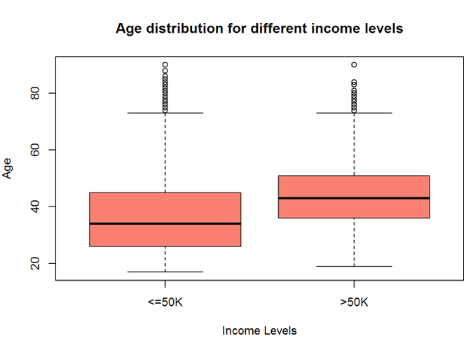
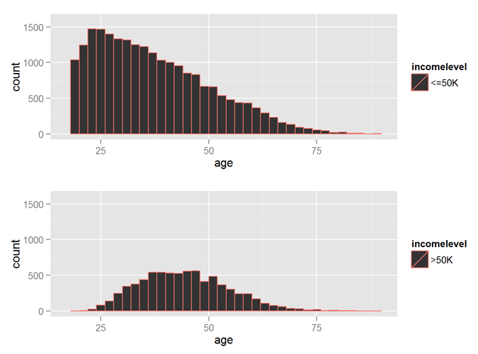
The Age variable has a wide range and variability. The distribution and mean are quite different for income level <=50K and >50K, implying that ‘age’ will be a good predictor of ‘incomelevel’.
summary (myCleanTrain$age)
##    Min. 1st Qu.  Median    Mean 3rd Qu.    Max.
##   17.00   28.00   37.00   38.44   47.00   90.00
boxplot (age ~ incomelevel, data = myCleanTrain,
         main = "Age distribution for different income levels",
         xlab = "Income Levels", ylab = "Age", col = "salmon")
incomeBelow50K = (myCleanTrain$incomelevel == "<=50K")
xlimit = c (min (myCleanTrain$age), max (myCleanTrain$age))
ylimit = c (0, 1600)

hist1 = qplot (age, data = myCleanTrain[incomeBelow50K,], margins = TRUE,
           binwidth = 2, xlim = xlimit, ylim = ylimit, colour = incomelevel)

hist2 = qplot (age, data = myCleanTrain[!incomeBelow50K,], margins = TRUE,
           binwidth = 2, xlim = xlimit, ylim = ylimit, colour = incomelevel)

grid.arrange (hist1, hist2, nrow = 2)
5.1.2 Explore the Years of Education Variable
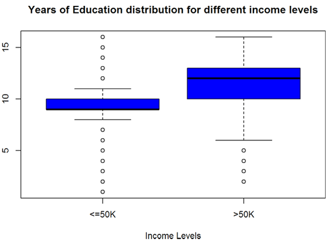
The Years of Education variable has good variability. The statistics are quite different for income level <=50K and >50K, implying that ‘educationnum’ will be a good predictor of ‘incomelevel’.
summary (myCleanTrain$educationnum)
##    Min. 1st Qu.  Median    Mean 3rd Qu.    Max.
##    1.00    9.00   10.00   10.12   13.00   16.00
boxplot (educationnum ~ incomelevel, data = myCleanTrain,
         main = "Years of Education distribution for different income levels",
         xlab = "Income Levels", ylab = "Years of Education", col = "blue")
5.1.3 Explore the Capital Gain and Capital Loss variables
The capital gain and capital loss variables do not show much variance for all income levels from the plots below. However, the means show a difference for the different levels of income. So these variables can be used for prediction.
nearZeroVar (myCleanTrain[, c("capitalgain", "capitalloss")], saveMetrics = TRUE)
##             freqRatio percentUnique zeroVar  nzv
## capitalgain  81.97033     0.3912207   FALSE TRUE
## capitalloss 148.11856     0.2983887   FALSE TRUE
summary (myCleanTrain[ myCleanTrain$incomelevel == "<=50K",
                       c("capitalgain", "capitalloss")])
##   capitalgain       capitalloss
##  Min.   :    0.0   Min.   :   0.00
##  1st Qu.:    0.0   1st Qu.:   0.00
##  Median :    0.0   Median :   0.00
##  Mean   :  148.9   Mean   :  53.45
##  3rd Qu.:    0.0   3rd Qu.:   0.00
##  Max.   :41310.0   Max.   :4356.00
summary (myCleanTrain[ myCleanTrain$incomelevel == ">50K",
                       c("capitalgain", "capitalloss")])
##   capitalgain     capitalloss
##  Min.   :    0   Min.   :   0.0
##  1st Qu.:    0   1st Qu.:   0.0
##  Median :    0   Median :   0.0
##  Mean   : 3938   Mean   : 193.8
##  3rd Qu.:    0   3rd Qu.:   0.0
##  Max.   :99999   Max.   :3683.0
5.1.4 Explore the Hours Per Week variable
The Hours Per Week variable has a good variability implying that ‘hoursperweek’ will be a good predictor of ‘incomelevel’.
summary (myCleanTrain$hoursperweek)
##    Min. 1st Qu.  Median    Mean 3rd Qu.    Max.
##    1.00   40.00   40.00   40.93   45.00   99.00
boxplot (hoursperweek ~ incomelevel, data = myCleanTrain,
         main = "Hours Per Week distribution for different income levels",
         xlab = "Income Levels", ylab = "Hours Per Week", col = "salmon")

nearZeroVar (myCleanTrain[, "hoursperweek"], saveMetrics = TRUE)
##   freqRatio percentUnique zeroVar   nzv
## 1  5.243194     0.3116504   FALSE FALSE
5.1.5 Explore the correlation between continuous variables
The below shows that there is no correlation between the continuous variables and that they are independent of each other.
corMat = cor (myCleanTrain[, c("age", "educationnum", "capitalgain", "capitalloss", "hoursperweek")])
diag (corMat) = 0 #Remove self correlations
corMat
##                     age educationnum capitalgain capitalloss hoursperweek
## age          0.00000000   0.04352609  0.08015423  0.06016548   0.10159876
## educationnum 0.04352609   0.00000000  0.12441600  0.07964641   0.15252207
## capitalgain  0.08015423   0.12441600  0.00000000 -0.03222933   0.08043180
## capitalloss  0.06016548   0.07964641 -0.03222933  0.00000000   0.05241705
## hoursperweek 0.10159876   0.15252207  0.08043180  0.05241705   0.00000000
5.2 Explore Categorical Variables
5.2.1 Exploring the Sex variable
Mostly the sex variable is not a good predictor, and so is the case for the income level prediction too. This variable will not be used for the model.
table (myCleanTrain[,c("sex", "incomelevel")])
##         incomelevel
## sex      <=50K  >50K
##   Female  8670  1112
##   Male   13984  6396
5.2.2 Exploring the work class, occupation, marital status, relationship and education variables
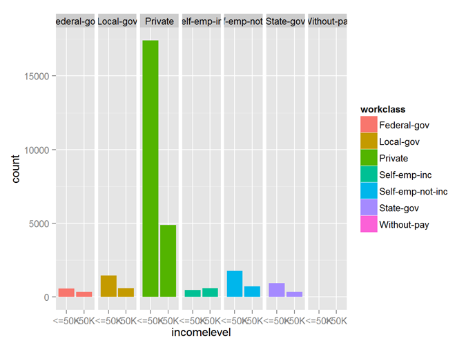
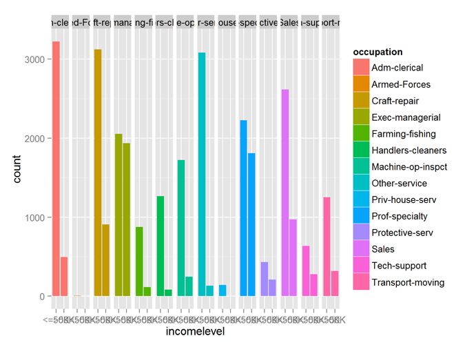
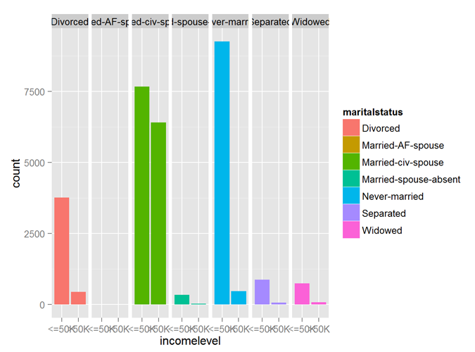
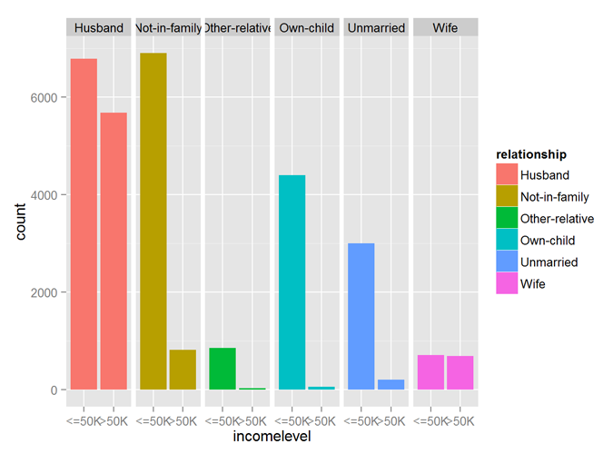
The variables workclass, occupation, maritalstatus, relationship all show good predictability of the incomelevel variable.
qplot (incomelevel, data = myCleanTrain, fill = workclass) + facet_grid (. ~ workclass)
qplot (incomelevel, data = myCleanTrain, fill = occupation) + facet_grid (. ~ occupation)
qplot (incomelevel, data = myCleanTrain, fill = maritalstatus) + facet_grid (. ~ maritalstatus)
qplot (incomelevel, data = myCleanTrain, fill = relationship) + facet_grid (. ~ relationship)
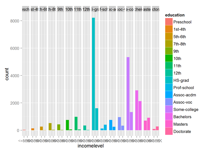
The education variable, however, needs to be reordered and marked an ordinal variable (ordered factor variable). The new ordinal variable also shows good predictability of incomelevel.
# Modify the levels to be ordinal
myCleanTrain$education = ordered (myCleanTrain$education,
    levels (myCleanTrain$education) [c(14, 4:7, 1:3, 12, 15, 8:9, 16, 10, 13, 11)])

print (levels (myCleanTrain$education))
##  [1] "Preschool"    "1st-4th"      "5th-6th"      "7th-8th"
##  [5] "9th"          "10th"         "11th"         "12th"
##  [9] "HS-grad"      "Prof-school"  "Assoc-acdm"   "Assoc-voc"
## [13] "Some-college" "Bachelors"    "Masters"      "Doctorate"
qplot (incomelevel, data = myCleanTrain, fill = education) + facet_grid (. ~ education)
5.2.3 Exploring the nativecountry variable
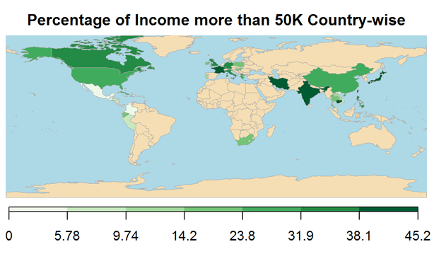
Plotting the percentage of Income more than USD 50000 nativecountry-wise, shows that nativecounty is a good predictor of incomelevel.
The names of the countries are cleaned for display on the world map. The code pertaining to these are now shown to keep the article concise.
## 40 codes from your data successfully matched countries in the map
## 0 codes from your data failed to match with a country code in the map
##      failedCodes failedCountries
## 204 codes from the map weren't represented in your data
5.3 Building the Prediction Model
Finally, down to building the prediction model, we will be using all the independent variables except the Sex variable to build a model that predicts the income level of an individual to be greater than USD 50000 or less than USD 50000 using Census data.
Since Census data is typical of weak predictors, the Boosting algorithm is used for this classification modeling.
I have also used Cross Validation (CV) where the training data is partitioned a specific number of times and separate boosted models are built on each. The resulting models are ensembled to arrive at final model. This helps avoid overfitting the model to the training data.
set.seed (32323)
trCtrl = trainControl (method = "cv", number = 10)

boostFit = train (incomelevel ~ age + workclass + education + educationnum +
                      maritalstatus + occupation + relationship +
                      race + capitalgain + capitalloss + hoursperweek +
                      nativecountry, trControl = trCtrl,
                  method = "gbm", data = myCleanTrain, verbose = FALSE)
The confusion matrix below shows an in-sample overall accuracy of ~86%, the sensitivity of ~88% and specificity of ~79%.
This implies that 86% of times, the model has classified the income level correctly, 88% of the times, the income level being less than or equal to USD 50000 in classified correctly and 79% of the times, the income level being greater than USD 50000 is classified correctly.
confusionMatrix (myCleanTrain$incomelevel, predict (boostFit, myCleanTrain))
## Confusion Matrix and Statistics
##
##           Reference
## Prediction <=50K  >50K
##      <=50K 21415  1239
##      >50K   2900  4608
##
##                Accuracy : 0.8628
##                  95% CI : (0.8588, 0.8666)
##     No Information Rate : 0.8061
##     P-Value [Acc > NIR] : < 2.2e-16
##
##                   Kappa : 0.6037
##  Mcnemar's Test P-Value : < 2.2e-16
##
##             Sensitivity : 0.8807
##             Specificity : 0.7881
##          Pos Pred Value : 0.9453
##          Neg Pred Value : 0.6137
##              Prevalence : 0.8061
##          Detection Rate : 0.7100
##    Detection Prevalence : 0.7511
##       Balanced Accuracy : 0.8344
##
##        'Positive' Class : <=50K
##
5.4 Validating the Prediction Model
The created prediction model is applied to the test data to validate the true performance. The test data is cleaned similar to the training data before applying the model.
##
## FALSE
## 15060
The cleaning is not shown to keep the case study concise. The cleaned test dataset has 15060 rows and 14 columns with no missing data.
The prediction model is applied on the test data. From the confusion matrix below the performance measures are out-of-sample overall accuracy of ~86%, sensitivity of ~88% and specificity of ~78%, which is quite similar to the in-sample performances
myCleanTest$predicted = predict (boostFit, myCleanTest)
confusionMatrix (myCleanTest$incomelevel, myCleanTest$predicted)
## Confusion Matrix and Statistics
##
##           Reference
## Prediction <=50K  >50K
##      <=50K 10731   629
##      >50K   1446  2254
##
##                Accuracy : 0.8622
##                  95% CI : (0.8566, 0.8677)
##     No Information Rate : 0.8086
##     P-Value [Acc > NIR] : < 2.2e-16
##
##                   Kappa : 0.5984
##  Mcnemar's Test P-Value : < 2.2e-16
##
##             Sensitivity : 0.8813
##             Specificity : 0.7818
##          Pos Pred Value : 0.9446
##          Neg Pred Value : 0.6092
##              Prevalence : 0.8086
##          Detection Rate : 0.7125
##    Detection Prevalence : 0.7543
##       Balanced Accuracy : 0.8315
##
##        'Positive' Class : <=50K
##
6. Executive Summary
During a data analytics exercise, it is very important to understand how the built model has performed with respect to a baseline model. This helps the analyst understand if there is really any value that the new model adds.
The baseline accuracy (here, accuracy of selection by random chance as there is no prior model) is 75% for income less than USD 50000 (sensitivity) and 25% for income more than USD 50000 (specificity) with an overall accuracy of 68% (Refer the skewed number of data sets for both the incomelevels in the cleaned test data).
The prediction model built using the boosting algorithm can predict a less than USD 50000 income level with 88% accuracy (sensitivity) and a more than USD 50000 income level with 78% accuracy (specificity) and an overall accuracy of 86%.
So the prediction model does perform better than the baseline model.
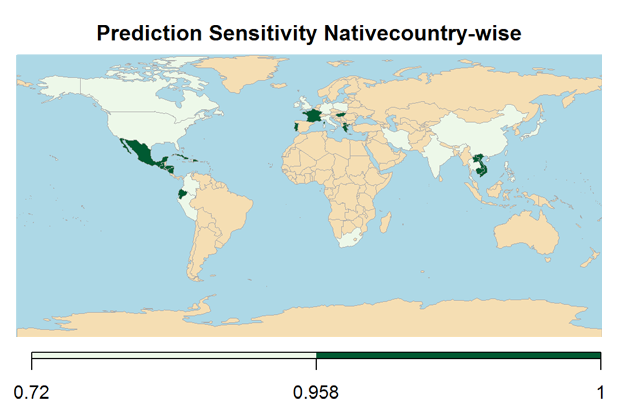
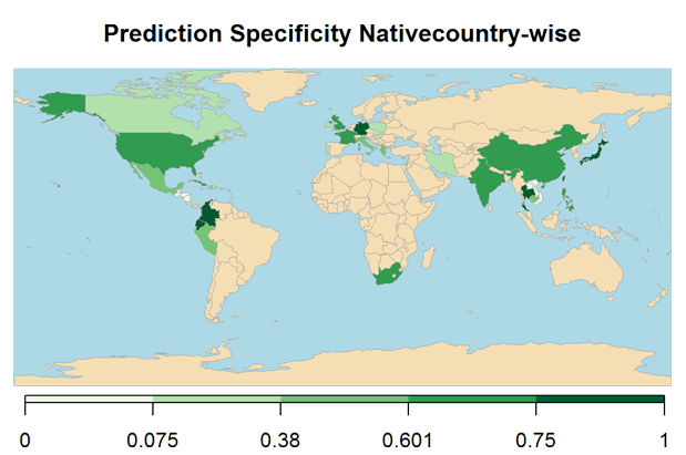
The below maps shows the overall prediction Overall Accuracy, Sensitivity and Specificity nativecountry-wise (For keeping the report concise, the computations for plotting the map are not shown).
## 39 codes from your data successfully matched countries in the map
## 0 codes from your data failed to match with a country code in the map
## 205 codes from the map weren't represented in your data




Hope this guide was helpful. Please feel free to leave your comments. Follow CloudxLab on Twitter to get updates on new blogs and videos.