We are glad to inform you that the TensorFlow is now available on CloudxLab. In this example, we will walk you through a basic tutorial on how to use TensorFlow.
What is TensorFlow?
TensorFlow is an Open Source Software Library for Machine Intelligence. It is developed and supported by Google and is being adopted very fast.
What is CloudxLab?
CloudxLab provides a real cloud-based environment for practicing and learn various tools. You can start learning right away by just signing up online.
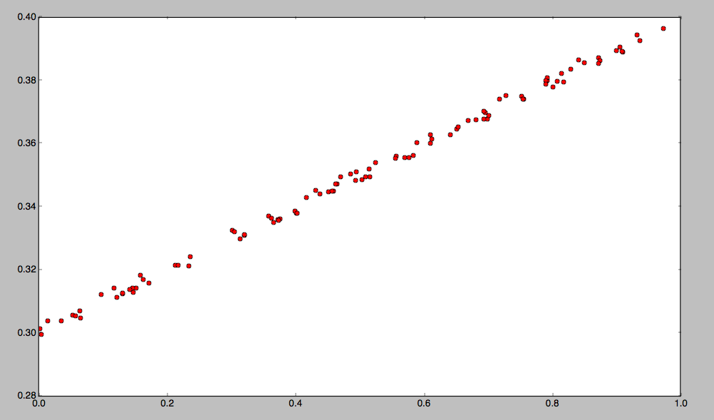
In this blog, we will go through a slight deviation of the first example of TensorFlow in the stepwise fashion as mentioned here. The objective of the exercise is to figure out the straight line that fits the given data. A line is characterized by the slope and intercept. In other words, we need to figure out the line that best suits the following points.
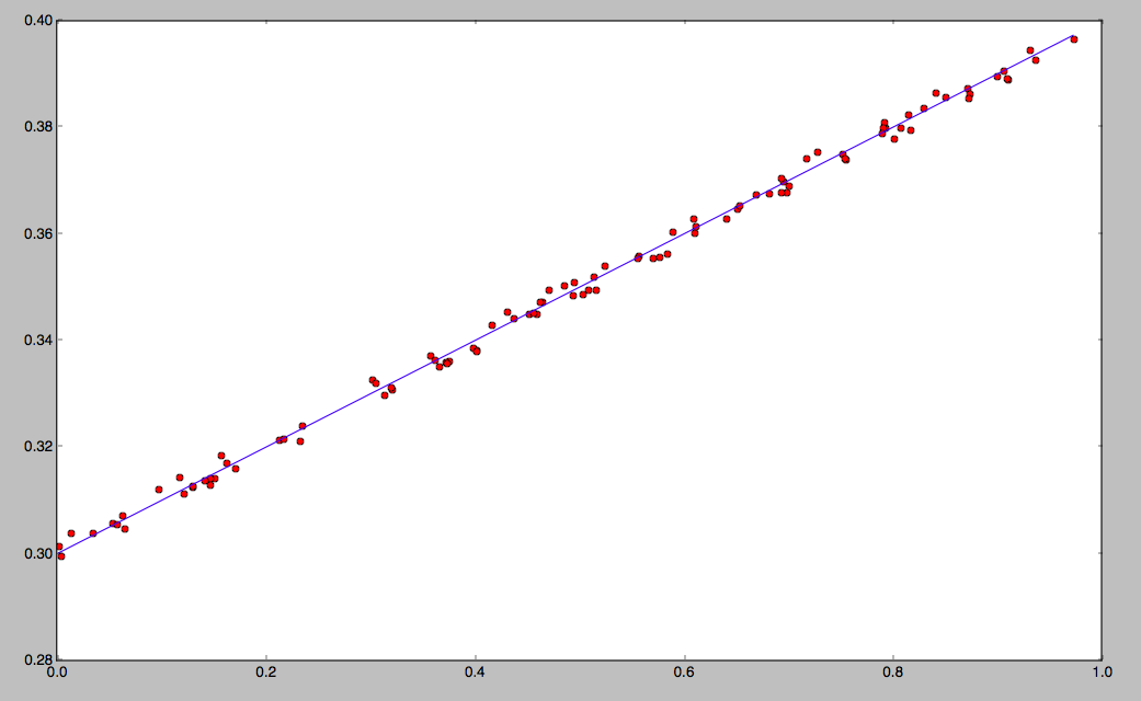
The end result of this exercise is to figure out the blue line as shown in the graph below:
Step 0: Login into cloudxLab
See this video to know how to login into the console.
Step 1: Start python interactive shell
Type “python” (without quotes) command on shell
Step 2: import libraries needed
import tensorflow as tf
import numpy as np
Step 3: Generate Some random data
x_data = np.random.rand(100).astype(np.float32)
def f(x):
   return x*0.1 + 0.3 + (np.random.rand()-0.5)/200
y_data = map(f, x_data)
Step 4: Define the variables that we need to figure out
W = tf.Variable(tf.random_uniform([1], -1.0, 1.0))
b = tf.Variable(tf.zeros([1]))
Step 5: Define relation between them – For simplicity we are assuming relation to be linear
y = W * x_data + b
Step 6: Define Loss function
# Minimize the mean squared errors.
loss = tf.reduce_mean(tf.square(y - y_data))
# For simplicity we are going to use standard Gradient Descent Optimizer
optimizer = tf.train.GradientDescentOptimizer(0.5)
train = optimizer.minimize(loss)
Step 8: Initialize
# Before starting, initialize the variables.  We will 'run' this first.
init = tf.initialize_all_variables()
Step 9: Launch
sess = tf.Session()
sess.run(init)
Step 10: Try to fit the line 250 times
for step in range(251):
    sess.run(train)
    #Print once every 20 iterations
    if step % 20 == 0:
        print(step, sess.run(W), sess.run(b))
Step 11: Understand the result
The above command will produce the results somewhat like this:
(0, array([-0.32815421], dtype=float32), array([ 0.71403891], dtype=float32))
(20, array([-0.02378235], dtype=float32), array([ 0.36488634], dtype=float32))
(40, array([ 0.0697251], dtype=float32), array([ 0.31596035], dtype=float32))
(60, array([ 0.09259172], dtype=float32), array([ 0.30399585], dtype=float32))
(80, array([ 0.09818359], dtype=float32), array([ 0.30107], dtype=float32))
(100, array([ 0.09955103], dtype=float32), array([ 0.30035451], dtype=float32))
(120, array([ 0.09988545], dtype=float32), array([ 0.30017954], dtype=float32))
(140, array([ 0.09996723], dtype=float32), array([ 0.30013674], dtype=float32))
(160, array([ 0.09998722], dtype=float32), array([ 0.30012628], dtype=float32))
(180, array([ 0.09999212], dtype=float32), array([ 0.30012372], dtype=float32))
(200, array([ 0.0999933], dtype=float32), array([ 0.3001231], dtype=float32))
(220, array([ 0.09999361], dtype=float32), array([ 0.30012295], dtype=float32))
(240, array([ 0.09999362], dtype=float32), array([ 0.30012295], dtype=float32))
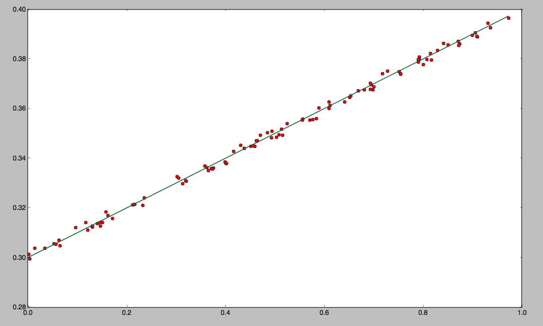
You can see that it has learned after 220 iterations that the best fit is W: [0.09999362] and b: [0.30012295]. So, the equation of the best line that fits the above points is y = x*0.09999362 + 0.30012295
If you plot this line along with the points, you would get a plot like this:
Practice TenserFlow now on CloudxLab