In the Part-1 we learned the following topics on Scala
Scala Features
Variables and Methods
Condition and Loops
Variables and Type Inference
Classes and Objects
Keeping up the same pace, we will learn the following topics in the 2nd part of the Scala series.
Functions Representation
Collections
Sequence and Sets
Tuples and Maps
Higher Order Functions
Build Tool – SBT
Functions Representation
We have already discussed functions. We can write a function in different styles in Scala. The first style is the usual way of defining a function.
scala> def add(x : int, y : int) : Int = {
         return x + y
       }
Please note that the return type is specified as Int.
In the second style, please note that the return type is omitted, also there is no “return” keyword. The Scala compiler will infer the return type of the function in this case.
scala> def add(x : int, y : int) = { //return type is inferred
         x + y //"return" keyword is optional
       }
If the function body has just one statement, then the curly braces are optional. In the third style, please note that there are no curly braces.
Welcome to the Scala tutorial. We will cover the Scala in two-part blog series. In this part, we will learn the following topics
Scala Features
Variables and Methods
Condition and Loops
Variables and Type Inference
Classes and Objects
For better understanding, do hands-on with this tutorial. We’ve made this post in such a way that the reader will find easy to follow the tutorial with hands-on.
Scala Features
Scala is a modern multi-paradigm programming language designed to express common programming patterns in a concise, elegant, and type-safe way.
It is a statically typed language. Which means it does type checking at compile-time as opposed to run-time. Let me give you an example to better understand this concept.
When we deploy jobs which will run for hours in production, we do not want to discover midway that the code has unexpected runtime errors. With Scala, you can be sure that your code will not give you unexpected errors while running in production.
Since Scala is statically typed we get performance and speed over dynamic languages.
How is Scala different than Java?
Unlike Java, in Scala, we do not have to write quite as much code to perform simple tasks and its syntax is very similar to other data-centric languages. You could say that Scala is the modified version of Java with less boilerplate code.
In the Part-1 we learned the following topics on Linux.
Linux Operating System
Linux Files & Process
The Directory Structure
Permissions
Process
Keeping up the same pace, we will learn the following topics in the 2nd part of the Linux series.
Shell Scripting
Networking
Files & Directories
Chaining Unix Commands
Pipes
Filters
Word Count Exercise
Special System commands
Environment variables
Writing first shell script
A shell script is a file containing a list of commands. Let’s create a simple command that prints two words:
1. Open a text editor to create a file myfirstscript.sh:
nano myfirstscript.sh
2. Write the following into the editor:
#!/bin/bash
name=linux
echo "hello $name world"
Note: In Unix, the extension doesn’t dictate the program to be used while executing a script. It is the first line of the script that would dictate which program to use. In the example above, the program is “/bin/bash” which is a Unix shell.
1. Press Ctrl +x to save and then “y” to exit
2. Now, by default, it would not have executable permission. You can make it executable like this:
We have started this series of tutorials for Linux which is divided into two blog posts. Each one of them will cover basic concepts with practical examples. Also, we have provided the quiz on some of the topics that you can attend for free.
In the first part of the series, we will learn the following topics in detail
Linux Operating System
Linux Files & Process
The Directory Structure
Permissions
Process
Introduction
Linux is a Unix like operating system. It is open source and free. We might sometimes use the word “Unix” instead of Linux.
A user can interact with Linux either using a ‘graphical interface’ or using the ‘command line interface’.
Learning to use the command line interface has a bigger learning curve than the graphical interface but the former can be used to automate very easily. Also, most of the server side work is generally done using the command line interface.
Linux Operating System
The operating system is made of three parts:
1. The Programs
A user executes programs. AngryBird is a program that gets executed by the kernel, for example. When a program is launched, it creates processes. Program or process will be used interchangeably.
2. The Kernel
The Kernel handles the main work of an operating system:
Allocates time & memory to programs
Handles File System
Responds to various Calls
3. The Shell
A user interacts with the Kernel via the Shell. The console as opened in the previous slide is the shell. A user writes instructions in the shell to execute commands. Shell is also a program that keeps asking you to type the name of other programs to run.
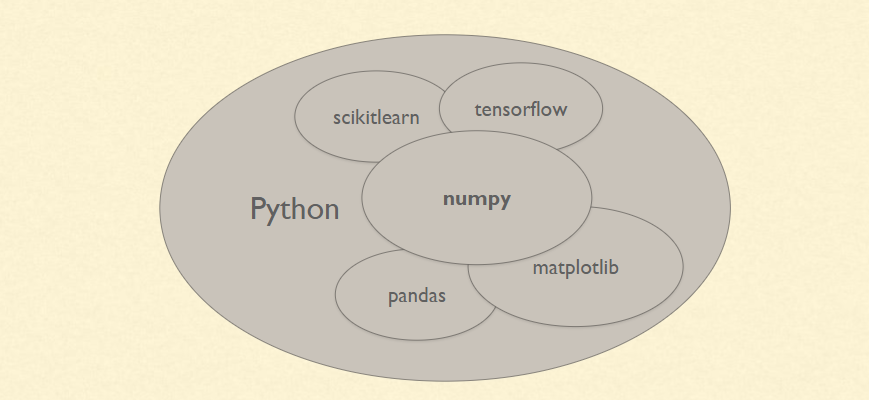
Python is increasingly being used as a scientific language. Matrix and vector manipulations are extremely important for scientific computations. Both NumPy and Pandas have emerged to be essential libraries for any scientific computation, including machine learning, in python due to their intuitive syntax and high-performance matrix computation capabilities.
In this post, we will provide an overview of the common functionalities of NumPy and Pandas. We will realize the similarity of these libraries with existing toolboxes in R and MATLAB. This similarity and added flexibility have resulted in wide acceptance of python in the scientific community lately. Topic covered in the blog are:
Overview of NumPy
Overview of Pandas
Using Matplotlib
This post is an excerpt from a live hands-on training conducted by CloudxLab on 25th Nov 2017. It was attended by more than 100 learners around the globe. The participants were from countries namely; United States, Canada, Australia, Indonesia, India, Thailand, Philippines, Malaysia, Macao, Japan, Hong Kong, Singapore, United Kingdom, Saudi Arabia, Nepal, & New Zealand.
Can a machine create quiz which is good enough for testing a person’s knowledge of a subject?
So, last Friday, we wrote a program which can create simple ‘Fill in the blank’ type questions based on any valid English text.
This program basically figures out sentences in a text and then for each sentence it would first try to delete a proper noun and if there is no proper noun, it deletes a noun.
We are using textblob which is basically a wrapper over NLTK – The Natural Language Toolkit, or more commonly NLTK, is a suite of libraries and programs for symbolic and statistical natural language processing for English written in the Python programming language.
In this post, we will learn how to configure tools required for CloudxLab’s Python for Machine Learning course. We will use Python 3 and Jupyter notebooks for hands-on practicals in the course. Jupyter notebooks provide a really good user interface to write code, equations, and visualizations.
Please choose one of the options listed below for practicals during the course.
GraphFrames is quite a useful library of spark which helps in bringing Dataframes and GraphX package together.
From the website of Graphframes:
GraphFrames is a package for Apache Spark which provides DataFrame-based Graphs. It provides high-level APIs in Scala, Java, and Python. It aims to provide both the functionality of GraphX and extended functionality taking advantage of Spark DataFrames. This extended functionality includes motif finding, DataFrame-based serialization, and highly expressive graph queries.
—
In this blog post, we will learn how to install Python packages on CloudxLab.
Step 1-
Create the virtual environment for your project. A virtual environment is a tool to keep the dependencies required by different projects in separate places, by creating virtual Python environments for them. Login to CloudxLab web console and create a virtual environment for your project.
First of all, let’s switch to python3 using:-
export PATH=/usr/local/anaconda/bin:$PATH
Now let’s create a directory and the virtual environment inside it.
You can run PySpark code in Jupyter notebook on CloudxLab. The following instructions cover 2.2, 2.3, 2.4 and 3.1 versions of Apache Spark.
What is Jupyter notebook?
The IPython Notebook is now known as the Jupyter Notebook. It is an interactive computational environment, in which you can combine code execution, rich text, mathematics, plots and rich media. For more details on the Jupyter Notebook, please see the Jupyter website.
Please follow below steps to access the Jupyter notebook on CloudxLab
To start python notebook, Click on “Jupyter” button under My Lab and then click on “New -> Python 3”
For accessing Spark, you have to set several environment variables and system paths. You can do that either manually or you can use a package that does all this work for you. For the latter, findspark is a suitable choice. It wraps up all these tasks in just two lines of code:
Here, we have used spark version 2.4.3. You can specify any other version too whichever you want to use. You can check the available spark versions using the following command-
!ls /usr/spark*
If you choose to do the setup manually instead of using the package, then you can access different versions of Spark by following the steps below:
If you want to access Spark 2.2, use below code:
import os
import sys

os.environ["SPARK_HOME"] = "/usr/hdp/current/spark2-client"
os.environ["PYLIB"] = os.environ["SPARK_HOME"] + "/python/lib"
# In below two lines, use /usr/bin/python2.7 if you want to use Python 2
os.environ["PYSPARK_PYTHON"] = "/usr/local/anaconda/bin/python"
os.environ["PYSPARK_DRIVER_PYTHON"] = "/usr/local/anaconda/bin/python"
sys.path.insert(0, os.environ["PYLIB"] +"/py4j-0.10.4-src.zip")
sys.path.insert(0, os.environ["PYLIB"] +"/pyspark.zip")
If you plan to use 2.3 version, please use below code to initialize
import os
import sys

os.environ["SPARK_HOME"] = "/usr/spark2.3/"
os.environ["PYLIB"] = os.environ["SPARK_HOME"] + "/python/lib"
# In below two lines, use /usr/bin/python2.7 if you want to use Python 2
os.environ["PYSPARK_PYTHON"] = "/usr/local/anaconda/bin/python"
os.environ["PYSPARK_DRIVER_PYTHON"] = "/usr/local/anaconda/bin/python"
sys.path.insert(0, os.environ["PYLIB"] +"/py4j-0.10.7-src.zip")
sys.path.insert(0, os.environ["PYLIB"] +"/pyspark.zip")
If you plan to use 2.4 version, please use below code to initialize
import os
import sys

os.environ["SPARK_HOME"] = "/usr/spark2.4.3"
os.environ["PYLIB"] = os.environ["SPARK_HOME"] + "/python/lib"
# In below two lines, use /usr/bin/python2.7 if you want to use Python 2
os.environ["PYSPARK_PYTHON"] = "/usr/local/anaconda/bin/python"
os.environ["PYSPARK_DRIVER_PYTHON"] = "/usr/local/anaconda/bin/python"
sys.path.insert(0, os.environ["PYLIB"] +"/py4j-0.10.7-src.zip")
sys.path.insert(0, os.environ["PYLIB"] +"/pyspark.zip")
Now, initialize the entry points of Spark: SparkContext and SparkConf (Old Style)
You can initialize spark in spark2 (or dataframe) way as follows:
# Entrypoint 2.x
from pyspark.sql import SparkSession
spark = SparkSession.builder.appName("Spark SQL basic example").enableHiveSupport().getOrCreate()
sc = spark.sparkContext
# Now you even use hive
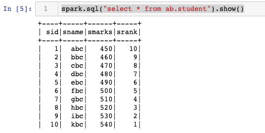
# Here we are querying the hive table student located in ab
spark.sql("select * from ab.student").show()
# it display something like this:
You can also initialize Spark 3.1 version, using the below code