As part of this blog post, I am going to walk you through how an Artificial Neural Network figures out a complex relationship in data by itself without much of our hand-holding. You should modify the data generation function and observe if it is able to predict the result correctly. I am going to use the Keras API of TensorFlow. Keras API makes it really easy to create Deep Learning models.
Machine learning is about computer figuring out relationships in data by itself as opposed to programmers figuring out and writing code/rules. Machine learning generally is categorized into two types: Supervised and Unsupervised. In supervised, we have the supervision available. And supervised learning is further classified into Regression and Classification. In classification, we have training data with features and labels and the machine should learn from this training data on how to label a record. In regression, the computer/machine should be able to predict a value – mostly numeric. An example of Regression is predicting the salary of a person based on various attributes: age, years of experience, the domain of expertise, gender.
The notebook having all the code is available here on GitHub as part of cloudxlab repository at the location deep_learning/tensorflow_keras_regression.ipynb . I am going to walk you through the code from this notebook here.
Generate Data: Here we are going to generate some data using our own function. This function is a non-linear function and a usual line fitting may not work for such a function
def myfunc(x):
    if x < 30:
        mult = 10
    elif x < 60:
        mult = 20
    else:
        mult = 50
    return x*mult
Let us check what does this function return.
print(myfunc(10))
print(myfunc(30))
print(myfunc(60))
It should print something like:
100
600
3000
Now, let us generate data. here x is a numpy array of input values. Let us import numpy library as np. Then using arange function we are generating values between 0 and 100 with a gap of 0.01. It generates a numpy array.
import numpy as np
x = np.arange(0, 100, .01)
To call a function repeatedly on a numpy array we first need to convert the function using vectorize. Afterwards, we are converting 1-D array to 2-D array having only one value in the second dimension – you can think of it as a table of data with only one column.
myfuncv = np.vectorize(myfunc)
y = myfuncv(x)
X = x.reshape(-1, 1)
Now, we have X representing the input data with single feature and y representing the output. We will now split this data into two parts: training set (X_train, y_train) and test set (X_test y_test). We are going make neural network learn from training data, and once it has learnt – how to produce y from X – we are going to test the model on the test set.
import sklearn.model_selection as sk

X_train, X_test, y_train, y_test = sk.train_test_split(X,y,test_size=0.33, random_state = 42)
Let us visualize how does our data looks like. Here, we are plotting only X_train vs y_train. You can try plotting X vs y, as well as, X_test vs y_test.
import matplotlib.pyplot as plt
plt.scatter(X_train,y_train)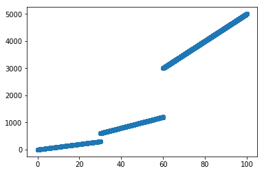
Let us now create a neural network and see if it can figure out the relationship. There are three steps involved: Create Neural Network, Train it and Test it.
Let us import TensorFlow libraries and check the version.
import tensorflow as tf
import numpy as np
print(tf.__version__)
It should print something like this:
‘1.10.0’
Now, let us create a neural network using Keras API of TensorFlow.
# Import the kera modules
from keras.layers import Input, Dense
from keras.models import Model

# This returns a tensor. Since the input only has one column
inputs = Input(shape=(1,))

# a layer instance is callable on a tensor, and returns a tensor
# To the first layer we are feeding inputs
x = Dense(32, activation='relu')(inputs)
# To the next layer we are feeding the result of previous call here it is h
x = Dense(64, activation='relu')(x)
x = Dense(64, activation='relu')(x)

# Predictions are the result of the neural network. Notice that the predictions are also having one column.
predictions = Dense(1)(x)

# This creates a model that includes
# the Input layer and three Dense layers
model = Model(inputs=inputs, outputs=predictions)
# Here the loss function is mse - Mean Squared Error because it is a regression problem.
model.compile(optimizer='rmsprop',
              loss='mse',
              metrics=['mse'])
Let us now train the model. First, it would initialize the weights of each neuron with random values and the using backpropagation it is going to tweak the weights in order to get the appropriate result. Here we are running the iteration 500 times and we are feeding 100 records of X at a time.
model.fit(X_train, y_train, epochs=500, batch_size=100) # starts trainingIt might show something like this on screen:
Epoch 1/500 6700/6700 [==============================] – 0s 36us/step – loss: 6084593.4888 – mean_squared_error: 6084593.4888
Epoch 2/500 6700/6700 [==============================] – 0s 13us/step – loss: 2762668.9375 – mean_squared_error: 2762668.9375
…..
Once we have trained the model. We can do predictions using the predict method of the model. In our case, this model should predict y using X. Let us test it over our test set. Plot the results.
# x_test = np.arange(0, 100, 0.02)
# X_test = x_test.reshape(-1, 1)
y_test = model.predict(X_test)
plt.scatter(X_test, y_test)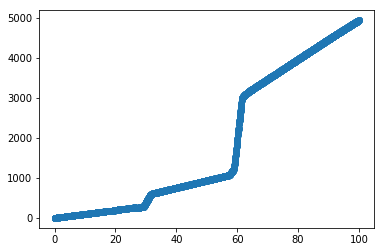
So, the predictions are very similar to the actual values.