In this duology of blogs, we will explore how to create a custom number plate reader. We will use a few machine learning tools to build the detector. An automatic number plate detector has multiple applications in traffic control, traffic violation detection, parking management etc. We will use the number plate detector as an exercise to try features in OpenCV, tensorflow object detection API, OCR, pytesseract
.
Machine Learning Tools Overview
We will use the following tools to build our application
- TensorFlow – One of the most popular open source libraries for machines learning, and supported by Google
- Tensorflow Object Detection API – We will use this API to create a model that will identify and localise the number plate. This API is an open-source framework built on top of TensorFlow. It lets us construct, train and deploy a variety of object detection models.
- SSD Inception v2 model – The SSD or single shot detector lets us detect and localise objects in an image with a single pass or a single shot. Tensorflow object detection API can use several models for object detection. We will use the SSD inception v2 model as it gives us a good balance of both accuracy and speed. You can find a list of all available models here.
- OpenCV – OpenCV or Open Computer Vision is the most popular tool for computer vision. It is written in C++, we will be using its Python extensions. OpenCV has a bunch of tools to manage pictures, videos and algorithms that manipulate images.
- Pytesseract – Pytesseract is a python wrapper for Tesseract an Optical Character Recogniser tool. It enables us to read text embedded in images.
- Python -We will write all code in Python 3.
- LabelImg – LabelImg is a graphical image annotation, which we will use in labelling our datasets.
Number Plate Reader Methodology
We will break down the task of building a custom number plate reader to the following
- Create a dataset of images with number plates
- Annotate the dataset with LabelImg
- Train an existing object detection model to detect number plates in a picture
- Extract the number plate using the trained model
- Run filters and cleanup of the picture
- Read the number plate using an OCR tool
- Identify shortcomings and explore methods to improve the model
We will cover the former 4 steps in this blog. The latter 3 will be covered in a later blog.
Creating the Dataset
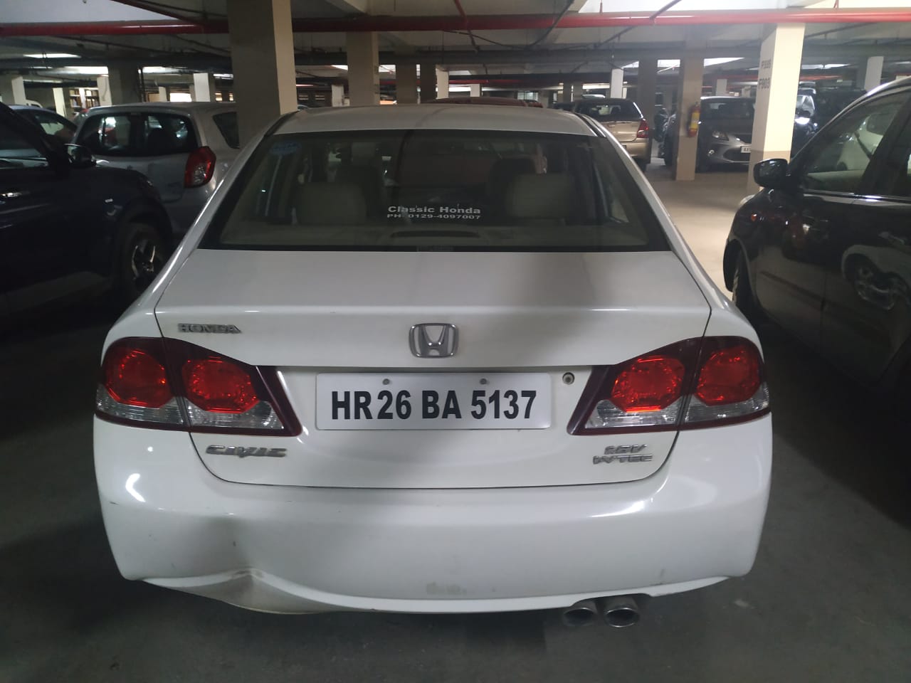
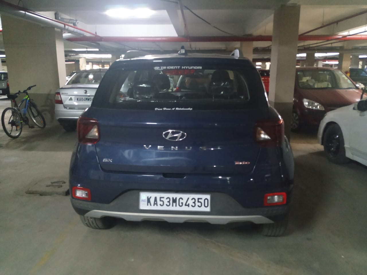
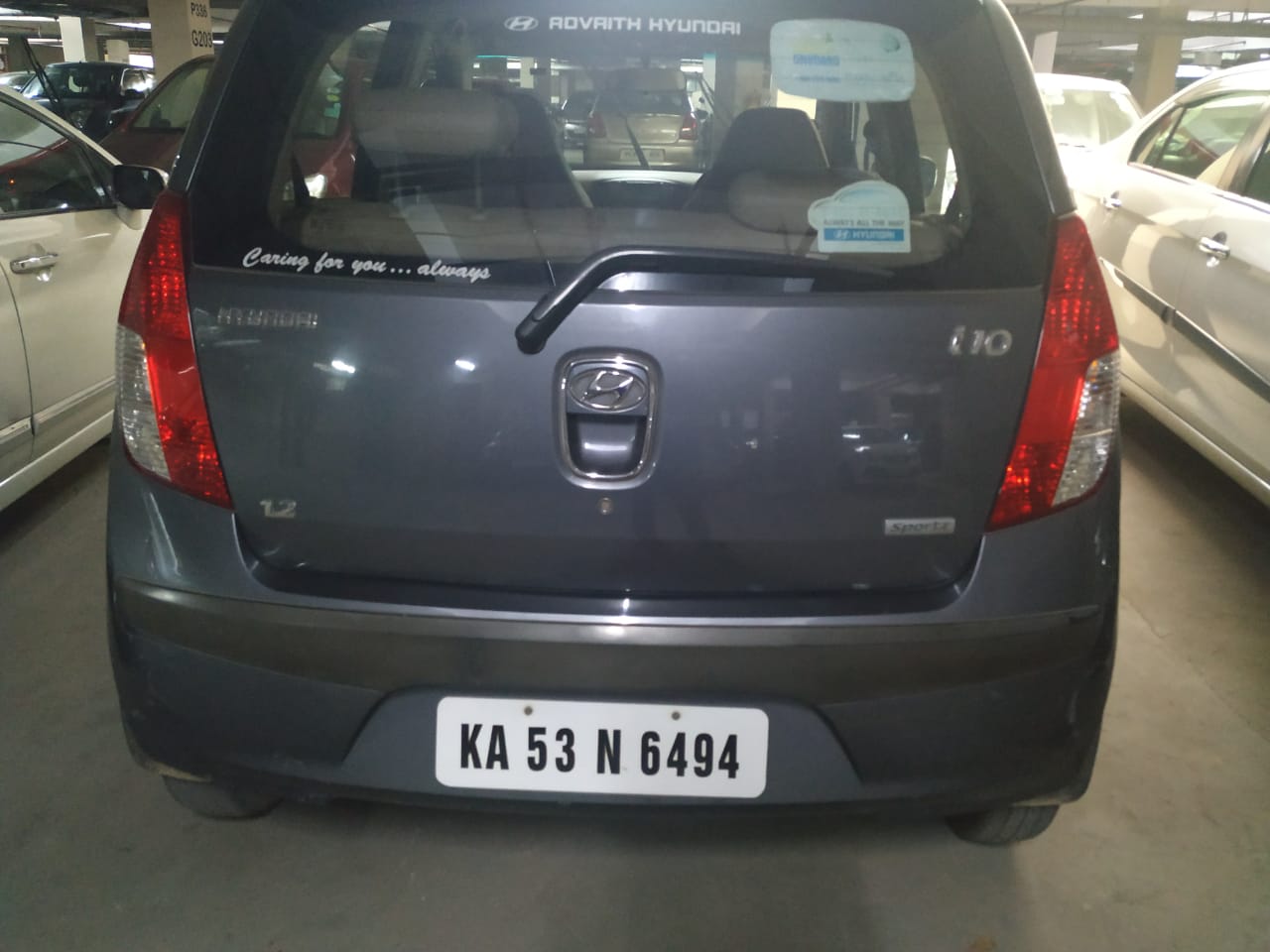
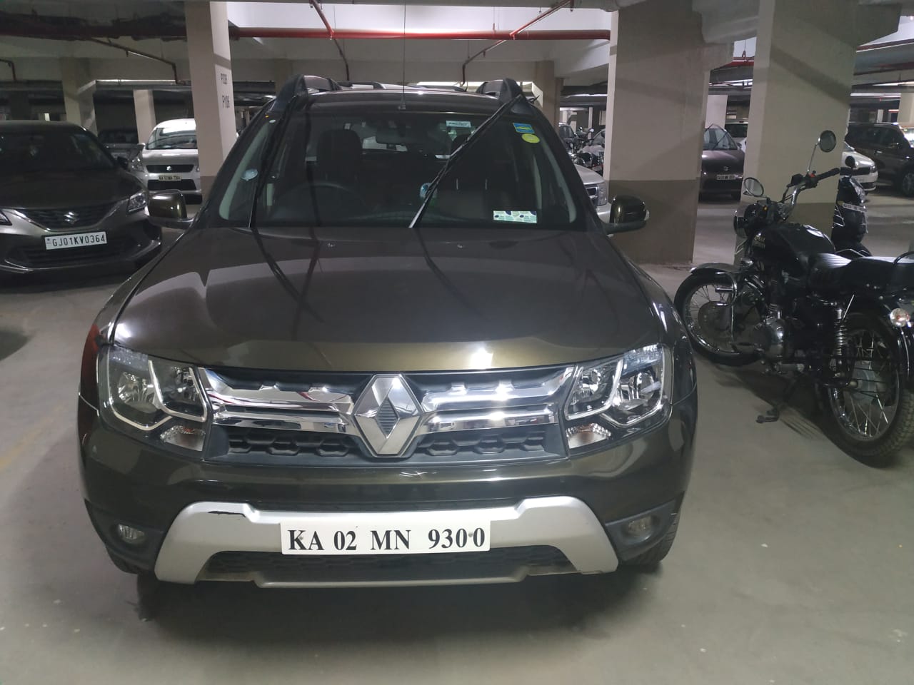
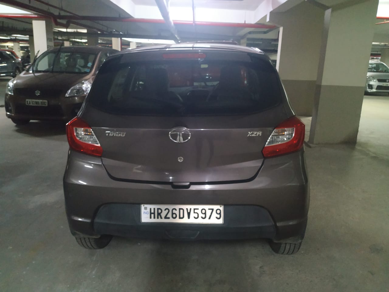
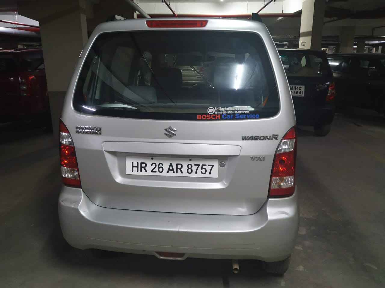
We can create a dataset on images with number plates like the ones above. You can take such photos with your mobile phone or scrape from the internet. Break the dataset into two directories – train and test. The train directory can have about 80% of the images and the test directory can have the remaining 20%.
I advise you to be very careful in this step. You should make sure that you shuffle the entire set and your test and train sets are random and not over-representative of a certain type of images. For e.g. you may choose images from multiple sources like mobile images, web scraped, cctv feed etc. If your test set or train set has more images from a single source like web scraping, you will see bad results. Make sure your test and train sets are randomised and as representative of the images you want to use in the end.
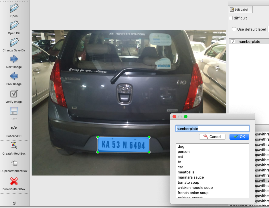
Annotating the Images
First create a new environment with virtualenv to manage the workflow. I strongly recommend using a virtualenvwrapper as it makes management of multiple python environments very easy.
pip3 install virtualenvwrapper
mkvirtualenv tf_obj
Install LabelImg following the instruction here. Choose the appropriate workflow based on your environment. Open LabelImg and open the directory containing the images and annotate them.

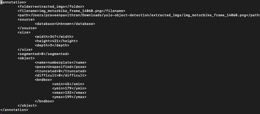
We will annotate both the train and test image sets. Enter the label as numberplate and choose Pascal/Voc as save format. Once your done, you will notice there are xml files associated with each picture. You can read the xml file and understand the parameters in the file. A sample xml file is below.
Training
Recommended Directory Structure
TensorFlow
├─ models
│   ├─ official
│   ├─ research
│   ├─ samples
│   └─ tutorials
└─ workspace
    └─ training_home
       ├─ annotations
       ├─ images
       │   ├─ test
       │   └─ train
       ├─ pre-trained-model
       ├─ training
       ├─ eval
       └─ trained-inference-graph
The images and xml files generated will be saved in the images directory. The test set and train set are kept images/test and images/train folders.
Install Tensorflow and Tensorflow Object Detection API
Tensorflow object detection API is a set of libraries that use TensorFlow. At the time of writing this blog tensorflow 2.0 was released but it did not support Tensorflow Object Detection yet. A key library tf.contrib was not part of tensorflow 2.0. For this exercise install version tf 1.15. Continue using the environment we created earlier.
- Tensorflow installation instructions: Note install tensorflow 1.15,
- Tensorflow Object Detection API instruction: This API models have to be downloaded and kept locally. We will store the models under the directory models as seen in the Recommended Directory Structure.
For your reference, we have provided the entire requirements.txt file here.
absl-py==0.9.0
ansiwrap==0.8.4
arrow==0.15.5
astor==0.8.1
astroid==2.3.3
astropy==3.2.3
attrs==19.3.0
backcall==0.1.0
bcolz==1.2.1
binaryornot==0.4.4
bleach==3.1.0
cachetools==4.0.0
certifi==2019.11.28
cffi==1.13.2
chardet==3.0.4
Click==7.0
cloud-tpu-profiler==1.15.0rc1
cloudpickle==1.2.2
colorama==0.4.3
configparser==4.0.2
confuse==1.0.0
cookiecutter==1.7.0
cryptography==1.7.1
cycler==0.10.0
Cython==0.29.15
daal==2019.0
datalab==1.1.5
decorator==4.4.1
defusedxml==0.6.0
dill==0.3.1.1
distro==1.0.1
docker==4.1.0
entrypoints==0.3
enum34==1.1.6
fairing==0.5.3
fsspec==0.6.2
future==0.18.2
gast==0.2.2
gcsfs==0.6.0
gitdb2==2.0.6
GitPython==3.0.5
google-api-core==1.16.0
google-api-python-client==1.7.11
google-auth==1.11.0
google-auth-httplib2==0.0.3
google-auth-oauthlib==0.4.1
google-cloud-bigquery==1.23.1
google-cloud-core==1.2.0
google-cloud-dataproc==0.6.1
google-cloud-datastore==1.10.0
google-cloud-language==1.3.0
google-cloud-logging==1.14.0
google-cloud-monitoring==0.31.1
google-cloud-spanner==1.13.0
google-cloud-storage==1.25.0
google-cloud-translate==2.0.0
google-compute-engine==20191210.0
google-pasta==0.1.8
google-resumable-media==0.5.0
googleapis-common-protos==1.51.0
grpc-google-iam-v1==0.12.3
grpcio==1.26.0
h5py==2.10.0
horovod==0.19.0
html5lib==1.0.1
htmlmin==0.1.12
httplib2==0.17.0
icc-rt==2020.0.133
idna==2.8
imageio==2.6.1
importlib-metadata==1.4.0
intel-openmp==2020.0.133
ipykernel==5.1.4
ipython==7.9.0
ipython-genutils==0.2.0
ipython-sql==0.3.9
ipywidgets==7.5.1
isort==4.3.21
jedi==0.16.0
Jinja2==2.11.0
jinja2-time==0.2.0
joblib==0.14.1
json5==0.8.5
jsonschema==3.2.0
jupyter==1.0.0
jupyter-aihub-deploy-extension==0.1
jupyter-client==5.3.4
jupyter-console==6.1.0
jupyter-contrib-core==0.3.3
jupyter-contrib-nbextensions==0.5.1
jupyter-core==4.6.1
jupyter-highlight-selected-word==0.2.0
jupyter-http-over-ws==0.0.7
jupyter-latex-envs==1.4.6
jupyter-nbextensions-configurator==0.4.1
jupyterlab==1.2.6
jupyterlab-git==0.9.0
jupyterlab-server==1.0.6
Keras==2.3.1
Keras-Applications==1.0.8
Keras-Preprocessing==1.1.0
keyring==10.1
keyrings.alt==1.3
kiwisolver==1.1.0
kubernetes==10.0.1
lazy-object-proxy==1.4.3
llvmlite==0.31.0
lxml==4.4.2
Markdown==3.1.1
MarkupSafe==1.1.1
matplotlib==3.0.3
mccabe==0.6.1
missingno==0.4.2
mistune==0.8.4
mkl==2019.0
mkl-fft==1.0.6
mkl-random==1.0.1.1
mock==3.0.5
more-itertools==8.1.0
nbconvert==5.6.1
nbdime==1.1.0
nbformat==5.0.4
networkx==2.4
nltk==3.4.5
notebook==6.0.3
numba==0.47.0
numpy==1.18.1
oauth2client==4.1.3
oauthlib==3.1.0
opencv-python==4.1.2.30
opt-einsum==3.1.0
packaging==20.1
pandas==0.25.3
pandas-profiling==1.4.0
pandocfilters==1.4.2
papermill==1.2.1
parso==0.6.0
pathlib2==2.3.5
pexpect==4.8.0
phik==0.9.8
pickleshare==0.7.5
Pillow==7.0.0
plotly==4.5.0
pluggy==0.13.1
poyo==0.5.0
prettytable==0.7.2
prometheus-client==0.7.1
promise==2.3
prompt-toolkit==2.0.10
protobuf==3.11.2
psutil==5.6.7
ptyprocess==0.6.0
py==1.8.1
pyarrow==0.15.1
pyasn1==0.4.8
pyasn1-modules==0.2.8
pycparser==2.19
pycrypto==2.6.1
pycurl==7.43.0
pydaal==2019.0.0.20180713
pydot==1.4.1
Pygments==2.5.2
pygobject==3.22.0
pylint==2.4.4
pyparsing==2.4.6
pyrsistent==0.15.7
pytest==5.3.4
pytest-pylint==0.14.1
python-apt==1.4.1
python-dateutil==2.8.1
pytz==2019.3
PyWavelets==1.1.1
pyxdg==0.25
PyYAML==5.3
pyzmq==18.1.1
qtconsole==4.6.0
requests==2.22.0
requests-oauthlib==1.3.0
retrying==1.3.3
rsa==4.0
scikit-image==0.15.0
scikit-learn==0.22.1
scipy==1.4.1
seaborn==0.9.1
SecretStorage==2.3.1
Send2Trash==1.5.0
simplegeneric==0.8.1
six==1.14.0
smmap2==2.0.5
SQLAlchemy==1.3.13
sqlparse==0.3.0
tbb==2019.0
tbb4py==2019.0
tenacity==6.0.0
tensorboard==1.15.0
tensorflow-datasets==1.2.0
tensorflow-estimator==1.15.1
tensorflow-gpu==1.15.2
tensorflow-hub==0.6.0
tensorflow-io==0.8.1
tensorflow-metadata==0.21.1
tensorflow-probability==0.9.0
tensorflow-serving-api-gpu==1.14.0
termcolor==1.1.0
terminado==0.8.3
testpath==0.4.4
textwrap3==0.9.2
tfds-nightly==1.0.1.dev201903050105
tornado==5.1.1
tqdm==4.42.0
traitlets==4.3.3
typed-ast==1.4.1
unattended-upgrades==0.1
uritemplate==3.0.1
urllib3==1.24.2
virtualenv==16.7.9
wcwidth==0.1.8
webencodings==0.5.1
websocket-client==0.57.0
Werkzeug==0.16.1
whichcraft==0.6.1
widgetsnbextension==3.5.1
witwidget-gpu==1.5.1
wrapt==1.11.2
zipp==1.1.0
The Label-Map file
The label-map file uniquely maps the labels in your model to integers. In our case we have only one label, so our label-map file will look like
item {
    id: 1
    name: 'numberplate'
}
We will call this file label-map.pbtxt. In case our model had more types of images we would have corresponding additional entries with unique integers mapping to the additional labels. We will keep this model in the annotations folder.
Creating the TF.Record
TensorFlow uses a binary format called TF.Record. Deep Learning uses large datasets, and storing the data in binary makes it efficient. It is more compact so it needs less disk for storage, and creates an efficient data pipeline to feed the training process. While working with datasets too large to store directly in memory, the training process only loads smaller segments or batches. TF.Records is highly optimised for TensorFlow and enables efficient data saving, loading, merging capabilities. Additionally, TF.Records simplifies processing of sequence data like time series and word encodings. For more details refer to this link.
There are two steps to create TF records. First we create csv files from the xml files, then we create the TF.record files. The code to generate the csv file is in the code block below. The code has the usage at the top. The input is the directory with the xml files and output is in the annotation directory.
"""
Usage:
# Create train data:
python xml_to_csv.py -i [PATH_TO_IMAGES_FOLDER]/train -o [PATH_TO_ANNOTATIONS_FOLDER]/train_labels.csv

# Create test data:
python xml_to_csv.py -i [PATH_TO_IMAGES_FOLDER]/test -o [PATH_TO_ANNOTATIONS_FOLDER]/test_labels.csv
"""

import os
import glob
import pandas as pd
import argparse
import xml.etree.ElementTree as ET


def xml_to_csv(path):
    """Iterates through all .xml files (generated by labelImg) in a given directory and combines them in a single Pandas datagrame.

    Parameters:
    ----------
    path : {str}
        The path containing the .xml files
    Returns
    -------
    Pandas DataFrame
        The produced dataframe
    """

    xml_list = []
    for xml_file in glob.glob(path + '/*.xml'):
        tree = ET.parse(xml_file)
        root = tree.getroot()
        for member in root.findall('object'):
            value = (root.find('filename').text,
                    int(root.find('size')[0].text),
                    int(root.find('size')[1].text),
                    member[0].text,
                    int(member[4][0].text),
                    int(member[4][1].text),
                    int(member[4][2].text),
                    int(member[4][3].text)
                    )
            xml_list.append(value)
    column_name = ['filename', 'width', 'height',
                'class', 'xmin', 'ymin', 'xmax', 'ymax']
    xml_df = pd.DataFrame(xml_list, columns=column_name)
    return xml_df


def main():
    # Initiate argument parser
    parser = argparse.ArgumentParser(
        description="Sample TensorFlow XML-to-CSV converter")
    parser.add_argument("-i",
                        "--inputDir",
                        help="Path to the folder where the input .xml files are stored",
                        type=str)
    parser.add_argument("-o",
                        "--outputFile",
                        help="Name of output .csv file (including path)", type=str)
    args = parser.parse_args()

    if(args.inputDir is None):
        args.inputDir = os.getcwd()
    if(args.outputFile is None):
        args.outputFile = args.inputDir + "/labels.csv"

    assert(os.path.isdir(args.inputDir))

    xml_df = xml_to_csv(args.inputDir)
    xml_df.to_csv(
        args.outputFile, index=None)
    print('Successfully converted xml to csv.')


if __name__ == '__main__':
    main()
After creating the csv files, we will use another script to create the TF.records. In the script below as you can see from the usage specified we take the csv files and create the record files. Note we use only one label here called numberplate. In case there are more, edit the FLAGS.label accordingly.
"""
Usage:

# Create train data:
python generate_tfrecord.py --label=<LABEL> --csv_input=<PATH_TO_ANNOTATIONS_FOLDER>/train_labels.csv  --output_path=<PATH_TO_ANNOTATIONS_FOLDER>/train.record

# Create test data:
python generate_tfrecord.py --label=<LABEL> --csv_input=<PATH_TO_ANNOTATIONS_FOLDER>/test_labels.csv  --output_path=<PATH_TO_ANNOTATIONS_FOLDER>/test.record
"""

from __future__ import division
from __future__ import print_function
from __future__ import absolute_import

import os
import io
import pandas as pd
import tensorflow as tf
import sys
sys.path.append("../../models/research")

from PIL import Image
from object_detection.utils import dataset_util
from collections import namedtuple, OrderedDict

flags = tf.app.flags
flags.DEFINE_string('csv_input', '', 'Path to the CSV input')
flags.DEFINE_string('output_path', '', 'Path to output TFRecord')
flags.DEFINE_string('label', '', 'Name of class label')
# if your image has more labels input them as
# flags.DEFINE_string('label0', '', 'Name of class[0] label')
# flags.DEFINE_string('label1', '', 'Name of class[1] label')
# and so on.
flags.DEFINE_string('img_path', '', 'Path to images')
FLAGS = flags.FLAGS


# TO-DO replace this with label map
# for multiple labels add more else if statements
def class_text_to_int(row_label):
    if row_label == FLAGS.label:  # 'numberplate':
        return 1
    # comment upper if statement and uncomment these statements for multiple labelling
    # if row_label == FLAGS.label0:
    #   return 1
    # elif row_label == FLAGS.label1:
    #   return 0
    else:
        None


def split(df, group):
    data = namedtuple('data', ['filename', 'object'])
    gb = df.groupby(group)
    return [data(filename, gb.get_group(x)) for filename, x in zip(gb.groups.keys(), gb.groups)]


def create_tf_example(group, path):
    with tf.gfile.GFile(os.path.join(path, '{}'.format(group.filename)), 'rb') as fid:
        encoded_jpg = fid.read()
    encoded_jpg_io = io.BytesIO(encoded_jpg)
    image = Image.open(encoded_jpg_io)
    width, height = image.size

    filename = group.filename.encode('utf8')
    image_format = b'jpg'
    # check if the image format is matching with your images.
    xmins = []
    xmaxs = []
    ymins = []
    ymaxs = []
    classes_text = []
    classes = []

    for index, row in group.object.iterrows():
        xmins.append(row['xmin'] / width)
        xmaxs.append(row['xmax'] / width)
        ymins.append(row['ymin'] / height)
        ymaxs.append(row['ymax'] / height)
        classes_text.append(row['class'].encode('utf8'))
        classes.append(class_text_to_int(row['class']))

    tf_example = tf.train.Example(features=tf.train.Features(feature={
        'image/height': dataset_util.int64_feature(height),
        'image/width': dataset_util.int64_feature(width),
        'image/filename': dataset_util.bytes_feature(filename),
        'image/source_id': dataset_util.bytes_feature(filename),
        'image/encoded': dataset_util.bytes_feature(encoded_jpg),
        'image/format': dataset_util.bytes_feature(image_format),
        'image/object/bbox/xmin': dataset_util.float_list_feature(xmins),
        'image/object/bbox/xmax': dataset_util.float_list_feature(xmaxs),
        'image/object/bbox/ymin': dataset_util.float_list_feature(ymins),
        'image/object/bbox/ymax': dataset_util.float_list_feature(ymaxs),
        'image/object/class/text': dataset_util.bytes_list_feature(classes_text),
        'image/object/class/label': dataset_util.int64_list_feature(classes),
    }))
    return tf_example


def main(_):
    writer = tf.python_io.TFRecordWriter(FLAGS.output_path)
    path = os.path.join(os.getcwd(), FLAGS.img_path)
    examples = pd.read_csv(FLAGS.csv_input)
    grouped = split(examples, 'filename')
    for group in grouped:
        tf_example = create_tf_example(group, path)
        writer.write(tf_example.SerializeToString())

    writer.close()
    output_path = os.path.join(os.getcwd(), FLAGS.output_path)
    print('Successfully created the TFRecords: {}'.format(output_path))


if __name__ == '__main__':
    tf.app.run()
Refer to the link for more details.
What is Transfer Training
We have converted the annotated images to a format compatible with tensorflow. In this section we will train an existing model to detect and localise a number plate in a picture. We will take an existing pre-trained model and feed it the annotated pictures from above. This process is called transfer training. The premise of transfer training is that the pre-existing model has already been extensively trained with a large set of images. So that model can already classify and detect a number of pictures. Tensorflow object detection API provides us with several models which have been pre-trained exhaustively with a large data set. By leveraging this learning we can get a working model that needs fewer number of images and fewer iterations. A list of these available models can be found in the model zoo.
MOdeL ZOO
We have multiple models in the model zoo; some are faster, others more accurate. Some of the models can even do segmentation, which identifies the pixels that make that object. For our application detecting bounding boxes is sufficient. The list of available models speed and accuracy measured and mAP (mean Average Precision) on the coco set is below. Higher the mAP, better the accuracy.
CONFIGURING the PIPELINE
We will use ssd_inception as it is a good balance between speed and accuracy. Since we use the pre-trained model as a starting point, download the pre-trained model from the model zoo. Decompress the file .tar.gz and store the contents in the directory pre-trained-model. We will now configure a pipeline for running the training. The pipeline will be configured with a config file. Samples of different config files can be found here. The config file for inception is here. We will now edit the file, to make it compatible for our data set. We have changed the following items in the file
- Change num_classes to 1 as we have only one class of objects.
- fine_tune_checkpoint: “pre-trained-model/model.ckpt” to point to the pretrained model
- input_path for both train and test sets.
- label_map to point to our label map in the annotations directory
- num_steps is set to 20000 which is sufficient for our use case
# SSD with Inception v2 configuration for MSCOCO Dataset.
# Users should configure the fine_tune_checkpoint field in the train config as
# well as the label_map_path and input_path fields in the train_input_reader and
# eval_input_reader. Search for "PATH_TO_BE_CONFIGURED" to find the fields that
# should be configured.

model {
  ssd {
    num_classes: 1    #Since we have only one class numberplates
    box_coder {
      faster_rcnn_box_coder {
        y_scale: 10.0
        x_scale: 10.0
        height_scale: 5.0
        width_scale: 5.0
      }
    }
    matcher {
      argmax_matcher {
        matched_threshold: 0.5
        unmatched_threshold: 0.5
        ignore_thresholds: false
        negatives_lower_than_unmatched: true
        force_match_for_each_row: true
      }
    }
    similarity_calculator {
      iou_similarity {
      }
    }
    anchor_generator {
      ssd_anchor_generator {
        num_layers: 6
        min_scale: 0.2
        max_scale: 0.95
        aspect_ratios: 1.0
        aspect_ratios: 2.0
        aspect_ratios: 0.5
        aspect_ratios: 3.0
        aspect_ratios: 0.3333
        reduce_boxes_in_lowest_layer: true
      }
    }
    image_resizer {
      fixed_shape_resizer {
        height: 300
        width: 300
      }
    }
    box_predictor {
      convolutional_box_predictor {
        min_depth: 0
        max_depth: 0
        num_layers_before_predictor: 0
        use_dropout: false
        dropout_keep_probability: 0.8
        kernel_size: 3
        box_code_size: 4
        apply_sigmoid_to_scores: false
        conv_hyperparams {
          activation: RELU_6,
          regularizer {
            l2_regularizer {
              weight: 0.00004
            }
          }
          initializer {
            truncated_normal_initializer {
              stddev: 0.03
              mean: 0.0
            }
          }
        }
      }
    }
    feature_extractor {
      type: 'ssd_inception_v2'
      min_depth: 16
      depth_multiplier: 1.0
      conv_hyperparams {
        activation: RELU_6,
        regularizer {
          l2_regularizer {
            weight: 0.00004
          }
        }
        initializer {
          truncated_normal_initializer {
            stddev: 0.03
            mean: 0.0
          }
        }
        batch_norm {
          train: true,
          scale: true,
          center: true,
          decay: 0.9997,
          epsilon: 0.001,
        }
      }
      override_base_feature_extractor_hyperparams: true
    }
    loss {
      classification_loss {
        weighted_sigmoid {
          anchorwise_output: true
        }
      }
      localization_loss {
        weighted_smooth_l1 {
          anchorwise_output: true
        }
      }
      hard_example_miner {
        num_hard_examples: 3000
        iou_threshold: 0.99
        loss_type: CLASSIFICATION
        max_negatives_per_positive: 3
        min_negatives_per_image: 0
      }
      classification_weight: 1.0
      localization_weight: 1.0
    }
    normalize_loss_by_num_matches: true
    post_processing {
      batch_non_max_suppression {
        score_threshold: 1e-8
        iou_threshold: 0.6
        max_detections_per_class: 100
        max_total_detections: 100
      }
      score_converter: SIGMOID
    }
  }
}

train_config: {
  batch_size: 24
  optimizer {
    rms_prop_optimizer: {
      learning_rate: {
        exponential_decay_learning_rate {
          initial_learning_rate: 0.004
          decay_steps: 800720
          decay_factor: 0.95
        }
      }
      momentum_optimizer_value: 0.9
      decay: 0.9
      epsilon: 1.0
    }
  }
  fine_tune_checkpoint: "pre-trained-model/model.ckpt"    # points to local starting point
  from_detection_checkpoint: true
  # Note: The below line limits the training process to 200K steps, which we
  # empirically found to be sufficient enough to train the pets dataset. This
  # effectively bypasses the learning rate schedule (the learning rate will
  # never decay). Remove the below line to train indefinitely.
  num_steps: 20000    #20 K steps is sufficient for us
  data_augmentation_options {
    random_horizontal_flip {
    }
  }
  data_augmentation_options {
    ssd_random_crop {
    }
  }
}

train_input_reader: {
  tf_record_input_reader {
    input_path: "annotations/train.record"   # Pointing to our training set
  }
  label_map_path: "annotations/label_map.pbtxt"   #Point to our labels
}

eval_config: {
  num_examples: 8000
  # Note: The below line limits the evaluation process to 10 evaluations.
  # Remove the below line to evaluate indefinitely.
  max_evals: 100
}

eval_input_reader: {
  tf_record_input_reader {
    input_path: "annotations/test.record"   #pointing to our eval set
  }
  label_map_path: "annotations/label_map.pbtxt"  #point to our label map
  shuffle: false
  num_readers: 1
  num_epochs: 1
}
We will keep the config pipeline in the training directory. To begin training and evaluation we will copy two files from the tensorflow object detection API to the directory training_home. The files are
- TensorFlow/models/research/object_detection/legacy/train.py
- TensorFlow/models/research/object_detection/legacy/eval.py
The following commands will launch training in the background, so the process will continue to run even if your session stops working.
nohup python3 train.py --train_dir=training/ --pipeline_config_path=train/ssd_inception_v2_coco.config > nohup_train.out 2>&1&
The command above runs training in the background. I found it easier to manage if the training is running this way. The logs can be monitored by running
tail -f nohup_train.outEvaluation and monitoring
As training runs, it saves checkpoint regularly in the directory training. If we have evaluation running in parallel, we can see how well each checkpoint runs. To run eval, the command is
nohup python eval.py --checkpoint_dir=training/ --eval_dir=eval/ --pipeline_config_path=train/ssd_inception_v2_coco.config > nohup_eval.out 2>&1&We can also run tensorboard, to monitor both the training and evaluation. We will run tensorboard on two different ports, so we can monitor both in parallel.
nohup tensorboard --logdir=train/ --port=8008 > nohup_tb_tr.out 2>&1&
nohup tensorboard --logdir=eval/ --port=6006 > nohup_tb_ev.out 2>&1&
Tensorboard runs an http server on the port so you can monitor it by going to it with any browser.
Exporting the Model
After the training is complete, we can export the trained model using the program from TensorFlow/models/research/object_detection/export_inference_graph.py to the training_home directory.
python export_inference_graph.py --input_type image_tensor --pipeline_config_path training/ssd_inception_v2_coco.config --trained_checkpoint_prefix training/model.ckpt-20000 --output_directory trained-inference-graphs/ssd_inception_output_inference_graph_number_plate_detector.pbNumber Plate Reader (Detector only)
We will now test the detector component of our number plate reader. Use the code below and change the path to MODEL_FILE and INPUT_FILE depending on your actuals.
import numpy as np
import tensorflow as tf
import cv2 as cv
import os
from os import listdir
from os.path import isfile, join


#Change PATH names to match your file paths for the model and INPUT_FILE'
MODEL_NAME='ssd_inception_output_inference_graph_v1.pb'
PATH_TO_FROZEN_GRAPH = MODEL_NAME + '/frozen_inference_graph.pb'
INPUT_FILE='test_images/img8.jpeg'


#Read the model from the file
with tf.gfile.FastGFile(PATH_TO_FROZEN_GRAPH, 'rb') as f:
    graph_def = tf.GraphDef()
    graph_def.ParseFromString(f.read())


#Create the tensorflow session
with tf.Session() as sess:

    sess.graph.as_default()
    tf.import_graph_def(graph_def, name='')
    # Read the input file
    img = cv.imread(INPUT_FILE)


    rows = img.shape[0]
    cols = img.shape[1]
    inp = cv.resize(img, (300, 300))
    inp = inp[:, :, [2, 1, 0]]  # BGR2RGB

    # Run the model
    out = sess.run([sess.graph.get_tensor_by_name('num_detections:0'),
                    sess.graph.get_tensor_by_name('detection_scores:0'),
                    sess.graph.get_tensor_by_name('detection_boxes:0'),
                    sess.graph.get_tensor_by_name('detection_classes:0')],
                   feed_dict={'image_tensor:0': inp.reshape(1, inp.shape[0], inp.shape[1], 3)})

    # Visualize detected bounding boxes.
    num_detections = int(out[0][0])
    # Iterate through all detected detections
    for i in range(num_detections):
        classId = int(out[3][0][i])

        score = float(out[1][0][i])
        bbox = [float(v) for v in out[2][0][i]]

        if score > 0.9:
            # Creating a box around the detected number plate
            x = int(bbox[1] * cols)
            y = int(bbox[0] * rows)
            right = int(bbox[3] * cols)
            bottom = int(bbox[2] * rows)
            cv.rectangle(img, (x, y), (right, bottom), (125, 255, 51), thickness=2)
            cv.imwrite('licence_plate_detected.png', img)
The output file of the number plate reader’s detector will look like this.

We have now learnt to use Tensorflow Object Detection API to build the number plate detector. In the second part we will now read the characters from this detected number plate.