Predicting Remaining Useful Life of a Machine

1.1 INTRODUCTION

The remaining useful life (RUL) is the length of time a machine is likely to operate before it requires repair or replacement. By taking RUL into account, engineers can schedule maintenance, optimize operating efficiency, and avoid unplanned downtime. For this reason, estimating RUL is a top priority in predictive maintenance programs.

Three are modeling solutions used for predicting the RUL which are mentioned below:

Regression: Predict the Remaining Useful Life (RUL), or Time to Failure (TTF).
Binary classification: Predict if an asset will fail within a certain time frame (e.g., Hours).
Multi-class classification: Predict if an asset will fail in different time windows: E.g., fails in window [1, w0] days; fails in the window [w0+1, w1] days; not fail within w1 days.

In this blog, I have covered binary classification and multi-class classification in the below sections.

1.2 DATASET

The dataset is taken from the actual turbine used in the ship, it consists of many features like sensor values, working hours, machine id, the actual life of the machine received from manufactures.

1.3 GENERAL

I am sharing my algorithm here. Even though this algorithm may not be of much use to you but it would give an idea of how to implement your own models for finding the remaining useful life of the machine.

Some of my learning are:

No firm provides the data of fault condition.
Figuring out how to customize LSTM is hard because the main documentation is messy.
Theory and Practical are two different things. The more hands-on you are, the higher are your chances of trying out an idea and thus iterating faster.

I applied Long Short-Term Memory (LSTM) because LSTM is used for time series problems. Since the dataset we have is time-dependent thus LSTM is the better model which can be used for prediction and it is a recurrent neural network that promises me to learn the long sequences of instances. It seems a perfect match for time series forecasting. In this project, you will see how to implement the LSTM forecast model for a one-step univariate time series forecasting problem.

In this blog we will go through the procedure to find the remaining useful life of the machine, it might help you to understand the process or procedure to complete your project.

2 PROCEDURE FOR PREDICTION

The procedure for finding the remaining useful life are given below:

Step 1: Import the dataset.

Step 2: Visualisation of dataset

Step 3: Co-relation between the features

Step 4: Labelling of training data by setting window length

Step 5: Normalization of data

Step 6: Labelling of test data based on the RUL

Step 7: Sequencing of data

Step 8: Preparation of model

Step 9: Fitting of model

Step 10: Validation of Model

Step 11: Prediction on test data

Step 12: Masking of test data

Step 13: Prediction on test data

2.1 Importing the dataset

The dataset taken for training and testing is taken from the data logger which is placed near to the machine on which prediction is to be made.

The sensors are installed on various assemblies and sub-assemblies of the turbine, the recorded sensor value is stored on a datalogger. The desired values are getting stored in a CSV file based on conditions and coding.

The dataset is imported by using the command as given below:

By the above code, data gets imported and the top 5 rows appear on the screen as shown below:

The number of rows that get displays on the screen can be changed by placing the desired value in the parathesis e.g. head(10).

2.2 Visualization of data

In this blog, I have visualized the data to see the variation of sensor values at a different instance. There are two ways in which variation may occur that are mentioned below:

1 If the rate of change in the sensor value is the same with respect to time then we see a linear line. In this case, the maintainer can find time to failure by taking multiplying factor hence don’t require any sort of predictions. But this case doesn’t happen in machines.

2. If the rate of change in the sensor values is different with respect to time then we get a non-linear line. In this case, predictive maintenance is applied which is explained in this blog.

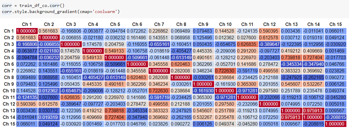
2.3 Co-relation between the features

In this blog, I co-related the values received from sensors for identifying which all sensors are showing critical changes.

2.4 Labelling of training data by setting window length

In this blog, we have labelled the RUL data since I am doing the classification of machine condition based on the values of RUL.

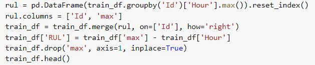
In the above image I have calculated the RUL of the machine then used that RUL for identifying the stage of the machine by defining the window length, I have set w1 as 450 and w0 as 300 based on normal condition, warning condition and critical condition values.

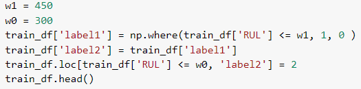
If RUL>w1 then the label will have value 1, if w1>RUL>300 then the label will be 2 and if RUL<w0 then the label will be 0.

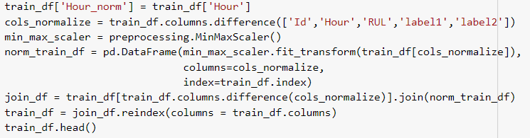
2.5 Normalization of data

In this blog, after labelling of training dataset I have normalized the data using MinMaxScalar. This is generally done we eliminate the change of losing the outliers and making all the values of sensors in a range of 0 to 1.

2.6 Labelling of testing data by setting window length

The same steps are to be followed as that of the training dataset only the difference will be of the dataset i.e. test dataset which is used for predictions.

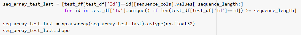
2.7: Sequencing of data

In this blog, I have applied predictions on time series forecasting thus sensor value will be read one by one, thus the dataset to be set in the proper sequence as it received one more use of sequencing is adding only those values which meet the window length considering no padding. I have taken a new matrix and then stored the value of test data into it.

2.8 Preparation of model

In this blog, I have taken 2 LSTM layers, 2 dropouts of 0.2 for eliminating overfitting, activation function as sigmoid as here we want where the machine is in running condition or is in faulty condition, optimizer as adam with binary crossentropy as the loss function.

2.9 Fitting of model

In this log, I have run the prepared model for 10 epochs with a batch size of 200 for better accuracy and validated the model by taking 5% of the dataset set for validation. I have also used callback for early stopping. Generally, we use callbacks for stopping the model training if validation loss increasing.

2.10 Validation of Model

In this blog, I have evaluated the model by calculating the score on a batch size of 200.

I got an accuracy of 98% which was sufficient for the model that can be used for prediction. It is observed that if we increase the batch size then accuracy increases but computation time also increases.

2.11 Prediction on test data

In this blog, I have taken the dataset of another day for testing the result. I have calculated the score, computed the confusion matrix. Using the confusion matrix I have calculated the precision, recall, F1- Score, accuracy which is shown below.

Referring above image, I figured out that there is some abrupt behaviour in predictions. There may be various reasons for the same. In my project, the dataset I used was of the running machine. I analysed the dataset and came to a conclusion that many values recorded in the datalogger were taken during the off condition of the machine where all the sensor values were at their default position giving no running status.

Thus, to resolve this problem I used masking technique which is described in the next section of this blog.

2.12 Masking of test data

In this blog, I have explained the masking technique in which I have masked the values of sensors which was recorded during the off condition of the machine. The limit for masking is taken as less than sequence length which fulfils our masking task.

2.13 Prediction of test data

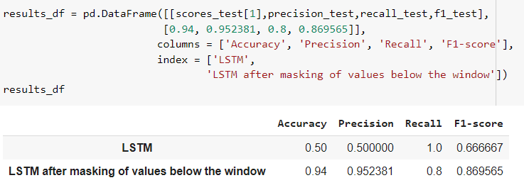
After masking the test dataset, I have again run the model, computed the confusion matrix. Using the confusion matrix I have calculated the precision, recall, F1- Score, accuracy.

The comparison between LSTM model without masking and with masking of the test dataset is shown below.